library(nimble)
## nimble version 1.0.1 is loaded.
## For more information on NIMBLE and a User Manual,
## please visit https://R-nimble.org.
##
## Note for advanced users who have written their own MCMC samplers:
##   As of version 0.13.0, NIMBLE's protocol for handling posterior
##   predictive nodes has changed in a way that could affect user-defined
##   samplers in some situations. Please see Section 15.5.1 of the User Manual.
##
##  次のパッケージを付け加えます: 'nimble'
##  以下のオブジェクトは 'package:stats' からマスクされています:
##
##     simulate
library(posterior)
## This is posterior version 1.4.1
##
##  次のパッケージを付け加えます: 'posterior'
##  以下のオブジェクトは 'package:stats' からマスクされています:
##
##     mad, sd, var
##  以下のオブジェクトは 'package:base' からマスクされています:
##
##     %in%, match
library(bayesplot)
## This is bayesplot version 1.10.0
## - Online documentation and vignettes at mc-stan.org/bayesplot
## - bayesplot theme set to bayesplot::theme_default()
##    * Does _not_ affect other ggplot2 plots
##    * See ?bayesplot_theme_set for details on theme setting
##
##  次のパッケージを付け加えます: 'bayesplot'
##  以下のオブジェクトは 'package:posterior' からマスクされています:
##
##     rhat
library(stringr)
library(ggplot2)The BUGS Book 11.8節 Bayesian nonparametric models の Example 11.8.1 Galaxy clustering: Dirichlet process mixuture models にあるモデルをNIMBLEに実装してみました。
Stanには松浦さんが移植しています(ノンパラベイズ(ディリクレ過程)の実装)。
準備
パッケージを読み込みます。
データ
The BUGS Bookのサポートページで配布されているExample-11.8.1-galaxy.odc をodcreadでテキストに変換して取り出しました。てもとのmacOS環境ではそのままではコンパイルが完了しなかったので、Makefileを修正する必要がありました。
データは、velocityが銀河の速度(×1000 km/h)、dens.xが速度の分布範囲、ndensがdens.xの要素数、Cがクラスター数の最大、nがvelocityの要素数です(でいいかな)。
velocity <- c( 9.172,  9.35,   9.483,  9.558,  9.775,
              10.227, 10.406, 16.084, 16.17,  18.419,
              18.552, 18.6,   18.927, 19.052, 19.07,
              19.33,  19.343, 19.349, 19.44,  19.473,
              19.529, 19.541, 19.547, 19.663, 19.846,
              19.856, 19.863, 19.914, 19.918, 19.973,
              19.989, 20.166, 20.175, 20.179, 20.196,
              20.215, 20.221, 20.415, 20.629, 20.795,
              20.821, 20.846, 20.875, 20.986, 21.137,
              21.492, 21.701, 21.814, 21.921, 21.96,
              22.185, 22.209, 22.242, 22.249, 22.314,
              22.374, 22.495, 22.746, 22.747, 22.888,
              22.914, 23.206, 23.241, 23.263, 23.484,
              23.538, 23.542, 23.666, 23.706, 23.711,
              24.129, 24.285, 24.289, 24.368, 24.717,
              24.99,  25.633, 26.96,  26.995, 32.065,
              32.789, 34.279)
dens.x <- seq(8, 35, 0.1)
ndens <- 271
C <- 20
n <- 82
モデル
NIMBLEのコードです。もとのBUGSコードはなぜかサンプリングがはじまらなかったのですが、NIMBLEマニュアルの10.3節 Stick-breaking modelを参考に、stick_breaking関数を使うように修正したら、うまく動作しました。
code <- nimbleCode({
  for (i in 1:n) {
    velocity[i] ~ dnorm(mu[i], tau[i])
    mu[i] <- mu.mix[group[i]]
    tau[i] <- tau.mix[group[i]]
    group[i] ~ dcat(pi[])
    for (j in 1:C) {
      gind[i, j] <- equals(j, group[i])
    }
  }
  for (j in 1:(C - 1)) {
    q[j] ~ dbeta(1, alpha)
  }
  pi[1:C] <- stick_breaking(q[1:(C - 1)])
  for (j in 1:C) {
    mu.mix[j] ~ dnorm(amu, mu.prec[j])
    mu.prec[j] <- bmu * tau.mix[j]
    tau.mix[j] ~ dgamma(aprec, bprec)
  }
  alpha <- 1
  amu ~ dnorm(0, 0.001)
  bmu ~ dgamma(0.5, 50)
  aprec <- 2
  bprec ~ dgamma(2, 1)
  K <- sum(cl[])
  for (j in 1:C) {
    sumind[j] <- sum(gind[, j])
    cl[j] <- step(sumind[j] - 1 + 0.001) # cluster j used in
                                         # this iteration
  }
  for (j in 1:ndens) {
    for (i in 1:C) {
      dens.cpt[i, j] <- pi[i] * sqrt(tau.mix[i] / (2 * 3.141592654)) *
                        exp(-0.5 * tau.mix[i] * (mu.mix[i] - dens.x[j])
                                              * (mu.mix[i] - dens.x[j]))
    }
    dens[j] <- sum(dens.cpt[, j])
  }
})
あてはめ
モデルをあてはめます。JAGSでThe BUGS BookのBUGSコードをあてはめるときにはとくに初期値を設定する必要はなかったのですが、NIMBLEではわりと細かく設定しないとうまく動作しません。
最後に、MCMCサンプルをposteriorパッケージのdrawsオブジェクトに変換します。さらに、その要約をsummaryオブジェクトに代入しておきます。
samp <- nimbleMCMC(code,
                    constants = list(C = C, n = n,
                                     ndens = ndens),
                    data = list(velocity = velocity,
                                dens.x = dens.x),
                    inits = list(amu = 0, bmu = 1,
                                 group = rep(1, n),
                                 gind = matrix(0, ncol = C, nrow = n),
                                 dens.cpt = matrix(1.0e-4,
                                                   ncol = ndens, nrow = C),
                                 cl = rep(1, C),
                                 q = rep(0.5, C),
                                 pi = rep(1 / C, C)),
                    monitors = c("K", "amu", "bmu", "cl", "dens",
                                 "mu.mix", "pi", "tau.mix"),
                    niter = 21000,
                    nburnin = 1000,
                    thin = 10,
                    nchains = 3,
                    samplesAsCodaMCMC = TRUE) |>
  as_draws()
## Defining model
## Building model
## Setting data and initial values
## Running calculate on model
##   [Note] Any error reports that follow may simply reflect missing values in model variables.
## Checking model sizes and dimensions
##   [Note] This model is not fully initialized. This is not an error.
##          To see which variables are not initialized, use model$initializeInfo().
##          For more information on model initialization, see help(modelInitialization).
## Checking model calculations
## [Note] NAs were detected in model variables: bprec, logProb_bprec, lifted_d1_over_bprec, tau.mix, logProb_tau.mix, mu.prec, lifted_d1_over_sqrt_oPmu_dot_prec_oBj_cB_cP_L12, tau, mu.mix, logProb_mu.mix, lifted_d1_over_sqrt_oPtau_oBi_cB_cP_L2, dens.cpt, dens, mu, logProb_velocity.
## Compiling
##   [Note] This may take a minute.
##   [Note] Use 'showCompilerOutput = TRUE' to see C++ compilation details.
## running chain 1...
## |-------------|-------------|-------------|-------------|
## |-------------------------------------------------------|
## running chain 2...
## |-------------|-------------|-------------|-------------|
## |-------------------------------------------------------|
## running chain 3...
## |-------------|-------------|-------------|-------------|
## |-------------------------------------------------------|
summary <- summary(samp)
収束診断
R-hat値をチェックします。rhatが大きい順に並べ替えています。
結果、R-hat値はどのパラメータでも1.1を下回っていました。
summary |>
  dplyr::arrange(desc(rhat))
## # A tibble: 354 × 10
##    variable    mean  median    sd     mad      q5    q95  rhat ess_bulk ess_tail
##    <chr>      <num>   <num> <num>   <num>   <num>  <num> <num>    <num>    <num>
##  1 mu.mix[… 19.8    20.0    5.90   3.91   9.59e+0 27.6    1.05     98.0    240.
##  2 pi[3]     0.157   0.0927 0.150  0.0919 1.18e-2  0.449  1.04    267.     689.
##  3 mu.mix[… 21.2    21.6    4.21   2.38   1.01e+1 26.9    1.04     60.8     60.3
##  4 tau.mix…  1.61    1.37   1.26   1.13   2.42e-1  3.85   1.03    133.     744.
##  5 mu.mix[… 19.6    19.9    7.97   6.23   9.43e+0 33.2    1.03     89.0    733.
##  6 tau.mix…  1.29    0.988  1.10   0.998  1.95e-1  3.29   1.03    116.    1387.
##  7 pi[2]     0.267   0.277  0.180  0.229  2.54e-2  0.548  1.03    158.     356.
##  8 pi[1]     0.355   0.372  0.202  0.181  3.32e-2  0.710  1.02    199.     313.
##  9 mu.mix[… 20.5    20.1    9.15  10.1    9.43e+0 33.5    1.02    123.    1238.
## 10 pi[4]     0.0943  0.0558 0.107  0.0513 5.74e-3  0.363  1.01    297.     478.
## # ℹ 344 more rows
軌跡
いくつかのパラメータで、MCMCの軌跡を見てみます。
pi[2]の末尾とかは微妙ですが、まあ、だいたいいいようです。
mcmc_trace(samp, pars = c("amu", "bmu", "pi[1]", "pi[2]"))
結果
クラスター数Kの事後分布の要約です。中央値は7、90%信用区間は4〜10でした。
summary |>
  dplyr::filter(variable == "K")
## # A tibble: 1 × 10
##   variable  mean median    sd   mad    q5   q95  rhat ess_bulk ess_tail
##   <chr>    <num>  <num> <num> <num> <num> <num> <num>    <num>    <num>
## 1 K         6.82      7  1.59  1.48     4    10  1.00     507.     631.
混合モデルの要素が含まれる確率です。点は平均値、線は90%信用区間です。
pi_est <- summary |>
  dplyr::filter(str_starts(variable, "pi")) |>
  dplyr::mutate(index = str_extract(variable, "[0-9]+") |>
                  as.numeric() |> as.factor())
ggplot(pi_est) +
  geom_point(aes(x = index, y = mean)) +
  geom_segment(aes(x = index, xend = index, y = q5, yend = q95)) +
  labs(x = "Component", y = "Probability")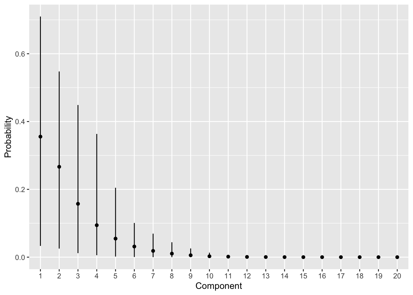
ディリクレ過程混合モデルにあてはめた銀河の速度の事後分布です。赤線が事後平均、赤色の領域が90%信用区間です。ヒストグラムは観測値のものです。
dens_est <- summary |>
  dplyr::filter(str_starts(variable, "dens")) |>
  dplyr::mutate(x = dens.x)
ggplot() +
  geom_histogram(data = data.frame(velocity = velocity),
                 mapping = aes(x = velocity, y = after_stat(density)),
                 bins = 30, fill = "gray") +
  geom_line(data = dens_est,
            mapping = aes(x = x, y = mean),
            colour = "red", linewidth = 1) +
  geom_ribbon(data = dens_est,
              mapping = aes(x = x, ymin = q5, ymax = q95),
              fill = "red", alpha = 0.3) +
  labs(x = "Galaxy velocity (x 1000 km/h)",
       y = "Probability density")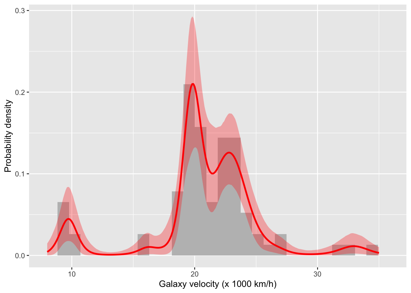
いずれも、The BUGS Bookにある結果(FIGURE 11.11)を再現できているようです。