間隔尺度変数の交互作用

第71回日本生態学会大会での粕谷さんの発表内容を自分でも確認してみました。回帰のとき、間隔尺度変数との交互作用がある変数は、間隔尺度変数のゼロの取り方が変わると、係数の値が変わるという話です。

準備

ライブラリの読み込みと乱数系列の設定です。

library(ggplot2)
set.seed(1234)

データ

ある植物の成長量\(y\)が説明変数\(x_1, x_2\)とそれらの交互作用に影響されるとします。 \(x_1\)は肥料の量のようなものを想定し、0〜100の値を取るとします。 間隔尺度変数の\(x_2\)は、30日間の摂氏0度以上の積算気温のようなものを想定し、450〜750の値を取るとし、それぞれ\(n\)(=20)段階で変化させるとします。 \(x_1\)の係数は\(\beta_1\)(=0.5)、\(x_2\)の係数は\(\beta_2\)(=0.1)、\(x_1\)と\(x_2\)の交互作用の係数は\(\beta_{12}\)(=0.001)とします。

また、目的変数\(y\)は、平均\(\mu = \beta + \beta_1 x1 + \beta_2 x_2 + \beta_{12} x_1 x_2\)、標準偏差\(\sigma\)(=10)の正規分布にしたがうとします。

n <- 20
x1 <- seq(0, 100, length = n)
x2 <- seq(450, 750, length = n)
df <- expand.grid(x1 = x1, x2 = x2)
beta1 <- 0.5
beta2 <- 0.1
beta12 <- 0.001
df$mu <- 10 + beta1 * df$x1 + beta2 * df$x2 + beta12 * df$x1 * df$x2
sigma <- 10
df$y <- rnorm(nrow(df), df$mu, sigma)

\(x_1\)と\(y\)との関係を図示します。

ggplot(df) +
  geom_point(aes(x = x1, y = y))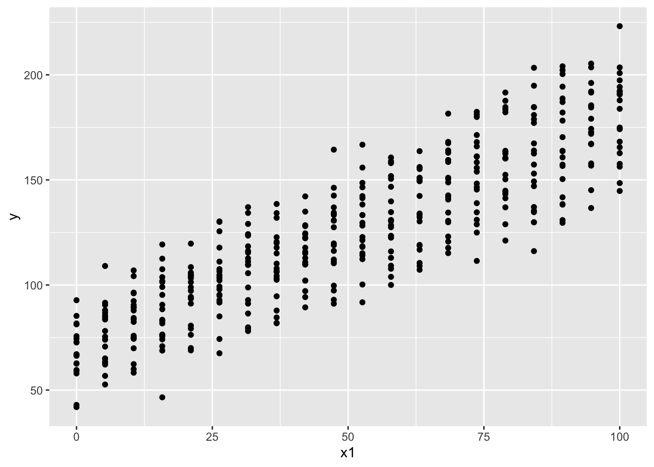

\(x_2\)と\(y\)との関係を図示します。

ggplot(df) +
  geom_point(aes(x = x2, y = y))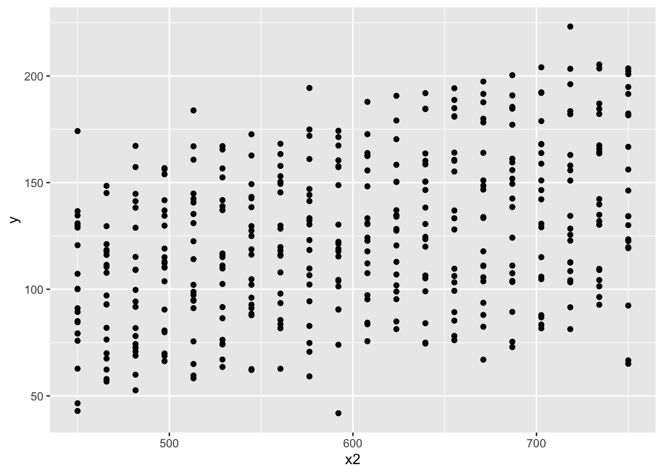

回帰

線形回帰の結果です。

lm(y ~ x1 + x2 + x1:x2, data = df) |>
  summary()
## 
## Call:
## lm(formula = y ~ x1 + x2 + x1:x2, data = df)
## 
## Residuals:
##     Min      1Q  Median      3Q     Max 
## -35.228  -6.402  -0.230   6.323  31.117 
## 
## Coefficients:
##              Estimate Std. Error t value Pr(>|t|)    
## (Intercept) 8.0104685  6.5191478   1.229     0.22    
## x1          0.4448570  0.1114579   3.991 7.83e-05 ***
## x2          0.1044998  0.0107423   9.728  < 2e-16 ***
## x1:x2       0.0010708  0.0001837   5.830 1.15e-08 ***
## ---
## Signif. codes:  0 '***' 0.001 '**' 0.01 '*' 0.05 '.' 0.1 ' ' 1
## 
## Residual standard error: 10.15 on 396 degrees of freedom
## Multiple R-squared:  0.9275, Adjusted R-squared:  0.927 
## F-statistic:  1689 on 3 and 396 DF,  p-value: < 2.2e-16

各係数の推定値はいずれも設定に近い値となりました。

間隔尺度変数の基準を変える

元の\(x_1\)は0℃以上の積算気温を想定していましたが、暖かさの指数にあわせて5℃以上の積算気温としてみます。30日間を想定しているので、150を元の値から引きます。

df$x2_2 <- df$x2 - 150

図示します。x軸のスケールが変わっただけです。

ggplot(df) +
  geom_point(aes(x = x2_2, y = y))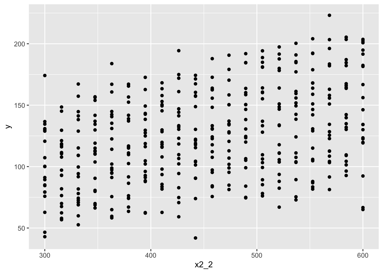

回帰してみます。

lm(y ~ x1 + x2_2 + x1:x2_2, data = df) |>
  summary()
## 
## Call:
## lm(formula = y ~ x1 + x2_2 + x1:x2_2, data = df)
## 
## Residuals:
##     Min      1Q  Median      3Q     Max 
## -35.228  -6.402  -0.230   6.323  31.117 
## 
## Coefficients:
##              Estimate Std. Error t value Pr(>|t|)    
## (Intercept) 2.369e+01  4.932e+00   4.802 2.23e-06 ***
## x1          6.055e-01  8.432e-02   7.181 3.46e-12 ***
## x2_2        1.045e-01  1.074e-02   9.728  < 2e-16 ***
## x1:x2_2     1.071e-03  1.837e-04   5.830 1.15e-08 ***
## ---
## Signif. codes:  0 '***' 0.001 '**' 0.01 '*' 0.05 '.' 0.1 ' ' 1
## 
## Residual standard error: 10.15 on 396 degrees of freedom
## Multiple R-squared:  0.9275, Adjusted R-squared:  0.927 
## F-statistic:  1689 on 3 and 396 DF,  p-value: < 2.2e-16

変えてはいない\(x_1\)の係数の値が大きくなりました。

基準変更その2

今度は、元の\(x_2\)から、ゼロが中央になるように、600を引いた値を新しい\(x_2\)とします。

df$x2_3 <- df$x2 - 600

図示してみます。やはりx軸のスケールが変わっただけです。

ggplot(df) +
  geom_point(aes(x = x2_3, y = y))

回帰してみます。

lm(y ~ x1 + x2_3 + x1:x2_3, data = df) |>
  summary()
## 
## Call:
## lm(formula = y ~ x1 + x2_3 + x1:x2_3, data = df)
## 
## Residuals:
##     Min      1Q  Median      3Q     Max 
## -35.228  -6.402  -0.230   6.323  31.117 
## 
## Coefficients:
##              Estimate Std. Error t value Pr(>|t|)    
## (Intercept) 7.071e+01  9.780e-01  72.298  < 2e-16 ***
## x1          1.087e+00  1.672e-02  65.026  < 2e-16 ***
## x2_3        1.045e-01  1.074e-02   9.728  < 2e-16 ***
## x1:x2_3     1.071e-03  1.837e-04   5.830 1.15e-08 ***
## ---
## Signif. codes:  0 '***' 0.001 '**' 0.01 '*' 0.05 '.' 0.1 ' ' 1
## 
## Residual standard error: 10.15 on 396 degrees of freedom
## Multiple R-squared:  0.9275, Adjusted R-squared:  0.927 
## F-statistic:  1689 on 3 and 396 DF,  p-value: < 2.2e-16

\(x_1\)の係数の値がさらに大きくなりました。

基準変更その3

次は、逆に600を足してみます。基準となる温度を-20℃とした場合に相当します。

df$x2_4 <- df$x2 + 600

図示して確認します。

ggplot(df) +
  geom_point(aes(x = x2_4, y = y))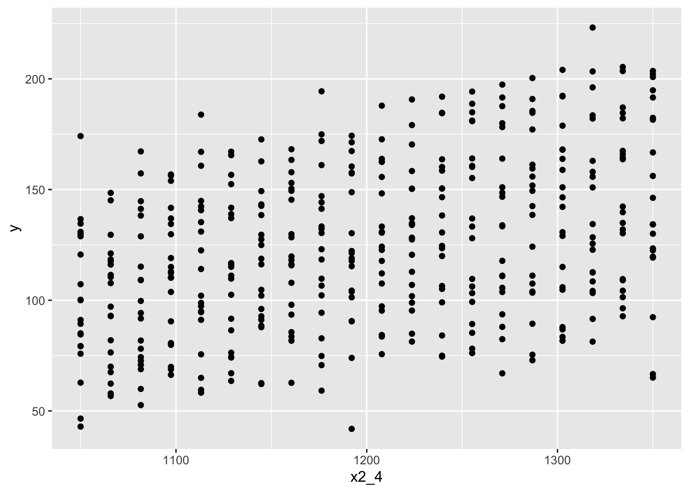

回帰の結果です。

lm(y ~ x1 + x2_4 + x1:x2_4, data = df) |>
  summary()
## 
## Call:
## lm(formula = y ~ x1 + x2_4 + x1:x2_4, data = df)
## 
## Residuals:
##     Min      1Q  Median      3Q     Max 
## -35.228  -6.402  -0.230   6.323  31.117 
## 
## Coefficients:
##               Estimate Std. Error t value Pr(>|t|)    
## (Intercept) -5.469e+01  1.293e+01  -4.230 2.90e-05 ***
## x1          -1.976e-01  2.210e-01  -0.894    0.372    
## x2_4         1.045e-01  1.074e-02   9.728  < 2e-16 ***
## x1:x2_4      1.071e-03  1.837e-04   5.830 1.15e-08 ***
## ---
## Signif. codes:  0 '***' 0.001 '**' 0.01 '*' 0.05 '.' 0.1 ' ' 1
## 
## Residual standard error: 10.15 on 396 degrees of freedom
## Multiple R-squared:  0.9275, Adjusted R-squared:  0.927 
## F-statistic:  1689 on 3 and 396 DF,  p-value: < 2.2e-16

今度は\(x_1\)の係数が（有意ではないですが）負になりました。

解説

数式で説明すると以下のようになります。元の回帰の平均は以下です。

\[ \beta + \beta_1 x1 + \beta_2 x_2 + \beta_{12} x_1 x_2 \]

\(x_2\)の基準を変えるとして、上の式に、\(x_2 = x'_2 + c\)を代入すると、以下のようになります。

\[ \beta + \beta_1 x1 + \beta_2 (x'_2 + c)+ \beta_{12} x_1 (x'_2 + c) \]

\[ = \beta + \beta_2 c + (\beta_1 + \beta_{12} c) x1 + \beta_2 x'_2 + \beta_{12} x_1 x'_2 \]

このように、\(x_2\)と交互作用項の係数は変わらないのに、\(x_1\)の係数（と切片）が変化します。

数式にしてみると一目瞭然なのですが、よく考えずに作業しているとハマりやすいところかもしれません。