library(nimble)
## nimble version 1.1.0 is loaded.
## For more information on NIMBLE and a User Manual,
## please visit https://R-nimble.org.
##
## Note for advanced users who have written their own MCMC samplers:
##   As of version 0.13.0, NIMBLE's protocol for handling posterior
##   predictive nodes has changed in a way that could affect user-defined
##   samplers in some situations. Please see Section 15.5.1 of the User Manual.
##
## 次のパッケージを付け加えます: 'nimble'
## 以下のオブジェクトは 'package:stats' からマスクされています:
##
##     simulate
## 以下のオブジェクトは 'package:base' からマスクされています:
##
##     declare
library(readr)
library(dplyr)
##
## 次のパッケージを付け加えます: 'dplyr'
## 以下のオブジェクトは 'package:stats' からマスクされています:
##
##     filter, lag
## 以下のオブジェクトは 'package:base' からマスクされています:
##
##     intersect, setdiff, setequal, union
library(tidyr)
library(stringr)
library(ggplot2)
library(posterior)
## This is posterior version 1.5.0
##
## 次のパッケージを付け加えます: 'posterior'
## 以下のオブジェクトは 'package:stats' からマスクされています:
##
##     mad, sd, var
## 以下のオブジェクトは 'package:base' からマスクされています:
##
##     %in%, match
library(bayesplot)
## This is bayesplot version 1.11.1
## - Online documentation and vignettes at mc-stan.org/bayesplot
## - bayesplot theme set to bayesplot::theme_default()
##    * Does _not_ affect other ggplot2 plots
##    * See ?bayesplot_theme_set for details on theme setting
##
## 次のパッケージを付け加えます: 'bayesplot'
## 以下のオブジェクトは 'package:posterior' からマスクされています:
##
##     rhat

set.seed(123)前の記事にひきつづき、松浦健太郎さんの“Bayesian Statistical Modeling with Stan, R, and Python”の11.6節にある、多変量正規分布の状態空間モデルをNIMBLEに移植してみました。
準備
ライブラリの読み込みと乱数の設定です。
データ
データを読み込んで整形します。サンプルコードと同様に、途中のデータを一部欠測とします。
data_url <- "https://raw.githubusercontent.com/MatsuuraKentaro/Bayesian_Statistical_Modeling_with_Stan_R_and_Python/master/chap11/input/data-eg2.csv"
d <- read_csv(data_url)
## Rows: 60 Columns: 3
## ── Column specification ────────────────────────────────────────────────────────
## Delimiter: ","
## dbl (3): Time, Weight, Bodyfat
##
## ℹ Use `spec()` to retrieve the full column specification for this data.
## ℹ Specify the column types or set `show_col_types = FALSE` to quiet this message.
T <- nrow(d)
t_obs2t <- c(1:20, 31:40, 51:60)
T_obs <- length(t_obs2t)
t_bf2t <- 21:30
T_bf <- length(t_bf2t)
Y_obs <- d[t_obs2t, c("Weight", "Bodyfat")] / 10
Y_bf <- d$Bodyfat[t_bf2t] / 10
モデル
NIMBLEのモデルです。NIMBLEでは独自の拡張として、Stanのモデルと同様に、LKJ相関分布のコレスキー因子を多変量正規分布のパラメータとして与えることができます。
相関行列と標準偏差ベクトルの掛け算をするuppertri_mult_diag関数は、マニュアルにあるものをそのままつかっています。
uppertri_mult_diag <- nimbleFunction(
  run = function(mat = double(2), vec = double(1)) {
    returnType(double(2))
    p <- length(vec)
    out <- matrix(nrow = p, ncol = p, init = FALSE)
    for(i in 1:p)
      out[ , i] <- mat[ , i] * vec[i]
    return(out)
  })

code <- nimbleCode({
  # observation model
  for (t in 1:T_obs) {
    mu_obs[t, 1:2] <- mu[t_obs2t[t], 1:2]
    Y_obs[t, 1:2] ~ dmnorm(mu_obs[t, 1:2],
                           cholesky = cov_chol_y[1:2, 1:2],
                           prec_param = 0)
  }
  for (t in 1:T_bf) {
    Y_bf[t] ~ dnorm(mu[t_bf2t[t], 2], sd = s_y_vec[2])
  }

  # system model
  for (t in 2:T) {
    mu[t, 1:2] ~ dmnorm(mu[t - 1, 1:2],
                        cholesky = cov_chol_mu[1:2, 1:2],
                        prec_param = 0)
  }
  mu[1, 1] ~ dnorm(0, sd = 10)
  mu[1, 2] ~ dnorm(0, sd = 10)

  # priors
  corr_chol_mu[1:2, 1:2] ~ dlkj_corr_cholesky(Nu, 2)
  corr_chol_y[1:2, 1:2] ~ dlkj_corr_cholesky(Nu, 2)
  cov_chol_mu[1:2, 1:2] <- uppertri_mult_diag(corr_chol_mu[1:2, 1:2],
                                              s_mu_vec[1:2])
  cov_chol_y[1:2, 1:2] <- uppertri_mult_diag(corr_chol_y[1:2, 1:2],
                                             s_y_vec[1:2])
  for (i in 1:2) {
    s_mu_vec[i] ~ dt(0, sigma = 0.05, df = 6)
    s_y_vec[i] ~ dt(0, sigma = 0.1, df = 6)
  }
})
実行
実行します。その前に、パラメータの初期値を生成するinits関数を定義しています。
繰り返し回数16万回で、そのうちの前半分の8万回をバーンインとしています。さらに20回ごとの間引きをつけていますが、これでも収束はなかなか難しいです。後でも見ますが、とくに標準偏差パラメータの収束が悪く、乱数によっては、大きな値で安定してしまう連鎖ができたりしてしまいます。
inits <- function() {
  list(mu = matrix(runif(T * 2, -2, 2), T, 2),
       s_mu_vec = runif(2, 0, 1),
       s_y_vec = runif(2, 0, 1),
       corr_chol_mu = matrix(runif(4, 0, 1), 2, 2),
       corr_chol_y = matrix(runif(4, 0, 1), 2, 2))
}

samp <- nimbleMCMC(code,
                   constants = list(T = T, T_obs = T_obs, T_bf = T_bf,
                                    t_obs2t = t_obs2t, t_bf2t = t_bf2t),
                   data =  list(Y_obs = Y_obs, Y_bf = Y_bf, Nu = 2),
                   inits = inits, setSeed = 11:13,
                   monitors = c("mu", "s_mu_vec", "s_y_vec"),
                   nchains = 3,
                   niter = 160000, nburnin = 80000, thin = 20,
                   samplesAsCodaMCMC = TRUE) |>
  as_draws()
## Defining model
## Building model
## Setting data and initial values
## Running calculate on model
##   [Note] Any error reports that follow may simply reflect missing values in model variables.
## Checking model sizes and dimensions
## Checking model calculations
## Compiling
##   [Note] This may take a minute.
##   [Note] Use 'showCompilerOutput = TRUE' to see C++ compilation details.
## Warning: Unknown or uninitialised column: `new`.
## Unknown or uninitialised column: `new`.
## Unknown or uninitialised column: `new`.
## running chain 1...
## |-------------|-------------|-------------|-------------|
## |-------------------------------------------------------|
## running chain 2...
## |-------------|-------------|-------------|-------------|
## |-------------------------------------------------------|
## running chain 3...
## |-------------|-------------|-------------|-------------|
## |-------------------------------------------------------|
結果
R-hatを確認します。大きい順に並べ替えて表示します。
samp |>
  summarise_draws() |>
  dplyr::arrange(desc(rhat)) |>
  dplyr::select(variable, rhat)
## # A tibble: 124 × 2
##    variable     rhat
##    <chr>       <dbl>
##  1 s_mu_vec[1]  1.25
##  2 s_y_vec[1]   1.07
##  3 s_mu_vec[2]  1.01
##  4 mu[35, 1]    1.01
##  5 mu[21, 2]    1.01
##  6 s_y_vec[2]   1.01
##  7 mu[27, 1]    1.01
##  8 mu[9, 1]     1.01
##  9 mu[26, 1]    1.01
## 10 mu[17, 1]    1.01
## # ℹ 114 more rowss_mu_vec[1]のR-hat値が1.1を超えてしまっています。
標準偏差パラメータのs_mu_vecとs_y_vecの軌跡を確認してみます。
mcmc_trace(samp, pars = c("s_mu_vec[1]", "s_mu_vec[2]",
                          "s_y_vec[1]", "s_y_vec[2]"))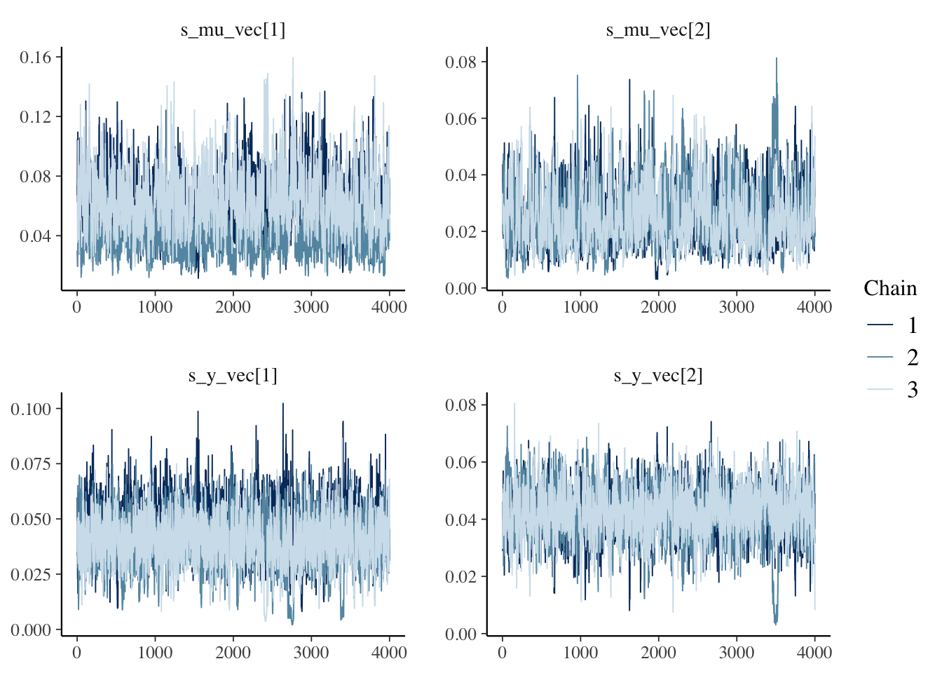
やはりs_mu_vec[1]の混ざり方がいまひとつです。Stanの結果と比較しても大きな値となっています。
グラフ表示
収束はいまひとつでしたが、状態muの推定値をみてみます。
summ <- samp |>
  summarise_draws(~quantile(.x, probs = c(0.025, 0.25, 0.5,
                                          0.75, 0.975)))
levels <- c("Weight", "Bodyfat")
mu <- summ |>
  dplyr::filter(str_detect(variable, "^mu")) |>
  dplyr::mutate_at(-1, ~ .x * 10) |>
  dplyr::bind_cols(data.frame(Time = c(1:T, 1:T),
                              Item = rep(levels, each = T))) |>
  dplyr::mutate(Item = factor(Item, levels = levels))

ggplot(mu, aes(x = Time)) +
  geom_ribbon(aes(ymin = `2.5%`, ymax = `97.5%`),
              fill = "gray80") +
  geom_ribbon(aes(ymin = `25%`, ymax = `75%`),
              fill = "gray50") +
  geom_line(aes(y = `50%`)) +
  labs(x = "Time (Day)", y = "Y") +
  facet_wrap(~Item, nrow = 2, scales = "free") +
  theme_bw()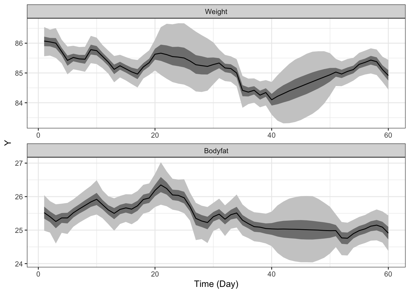
muの推定値はだいたいStanの結果と同様となっていました。