library(cmdstanr)
## This is cmdstanr version 0.8.1
## - CmdStanR documentation and vignettes: mc-stan.org/cmdstanr
## - CmdStan path: /usr/local/cmdstan
## - CmdStan version: 2.35.0
library(bayesplot)
## This is bayesplot version 1.11.1
## - Online documentation and vignettes at mc-stan.org/bayesplot
## - bayesplot theme set to bayesplot::theme_default()
##    * Does _not_ affect other ggplot2 plots
##    * See ?bayesplot_theme_set for details on theme setting
library(ggplot2)

qgl <- read.csv(url("https://raw.githubusercontent.com/iwanami-datascience/vol1/master/ito/Qglauca.csv"))
register_knitr_engine()空間自己相関をとりいれたStanのモデルは、 Max Josephさんの“Exact sparse CAR models in Stan”、Mitzi Morrisさんの“Spatial Models in Stan: Intrinsic Auto-Regressive Models for Areal Data”がStanのCase Studiesに掲載されています。また松浦健太郎さんの“Bayesian Statistical Modeling with Stan, R, and Python”の第12章でも紹介されています。
今回はこのうちMitzi MorrisさんのICAR (Intrinsic Conditional Auto-Regressive) モデルを使ってみたいと思います。
データ
岩波データサイエンスVol.1で使用した、10×20のグリッド中のアラカシの株数データを使用します。
図示
まずはデータをプロットします。
ggplot(qgl, aes(x = X, y = Y)) +
  geom_tile(aes(fill = N)) +
  scale_y_reverse(breaks = c(0, 5, 10)) +
  scale_fill_gradient(name = "株数", low = "grey90", high = "grey10") +
  coord_fixed(ratio = 1) +
  theme_bw(base_family = "IPAexGothic")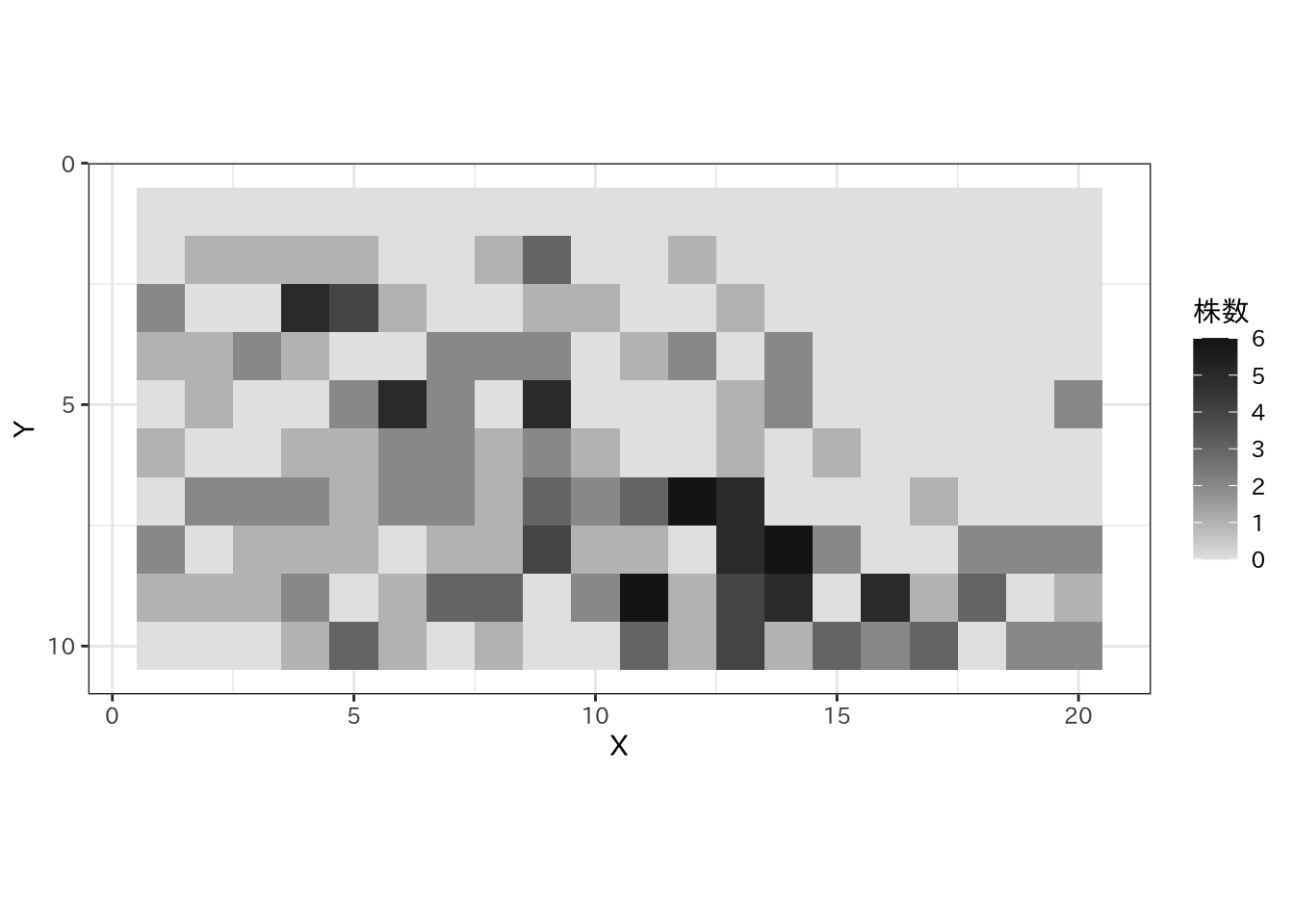
隣接リストの作成
隣接リストを作成します。このモデルでは、node1とnode2 (node1 < node2) に隣接関係を記述していきます。
n.x <- max(qgl$X)
n.y <- max(qgl$Y)
n_edges <- (2 * 4 +
            3 * (2 * (n.x - 2) + (2 * (n.y - 2))) +
            4 * (n.x - 2) * (n.y - 2)) / 2
node1 <- node2 <- rep(0, n_edges)

i <- 1
for (j in 1:(n.x - 1)) {
  for (k in 1:(n.y - 1)) {
    node1[i + 1] <- node1[i] <- n.y * (j - 1) + k
    node2[i] <- n.y * (j - 1) + k + 1
    node2[i + 1] <- n.y * j + k
    i <- i + 2
  }
}
# right side
for (j in 1:(n.y - 1)) {
  node1[i] <- n.y * (n.x - 1) + j
  node2[i] <- n.y * (n.x - 1) + j + 1
  i <- i + 1
}
# bottom side
for (j in 1:(n.x - 1)) {
  node1[i] <- n.y * j
  node2[i] <- n.y * (j + 1)
  i <- i + 1
}
モデル
モデルです。説明変数は今回は用いないので、元のモデルにあったbeta1とxは消去してあります。その他はそのままです。
beta0が切片、phiが空間自己相関、thetaが不均一性のパラメータです。
/*
 * from Spatial Models in Stan: Intrinsic Auto-Regressive Models for Areal Data
 * https://mc-stan.org/users/documentation/case-studies/icar_stan.html
 */

data {
  int<lower=0> N;
  int<lower=0> N_edges;
  array[N_edges] int<lower=1, upper=N> node1; // node1[i] adjacent to node2[i]
  array[N_edges] int<lower=1, upper=N> node2; // and node1[i] < node2[i]
  array[N] int<lower=0> Y; // count outcomes
}

parameters {
  real beta0; // intercept

  real<lower=0> tau_theta; // precision of heterogeneous effects
  real<lower=0> tau_phi; // precision of spatial effects

  vector[N] theta; // heterogeneous effects
  vector[N] phi; // spatial effects
}

transformed parameters {
  real<lower=0> sigma_theta = inv(sqrt(tau_theta)); // convert precision to sigma
  real<lower=0> sigma_phi = inv(sqrt(tau_phi)); // convert precision to sigma
}

model {
  Y ~ poisson_log(beta0 + phi * sigma_phi
                  + theta * sigma_theta);

  target += -0.5 * dot_self(phi[node1] - phi[node2]);
  sum(phi) ~ normal(0, 0.001 * N); // equivalent to mean(phi) ~ normal(0,0.001)

  beta0 ~ normal(0, 5);
  theta ~ normal(0, 1);
  tau_theta ~ gamma(3.2761, 1.81); // Carlin WinBUGS priors
  tau_phi ~ gamma(1, 1); // Carlin WinBUGS priors
}

generated quantities {
  vector[N] mu = exp(beta0 + phi * sigma_phi
                     + theta * sigma_theta);
}
あてはめ
cmdstanr経由でStanを実行してモデルをあてはめます。Stanのモデルはmodelオブジェクトにいれておいてあります。
stan_data <- list(N = nrow(qgl), N_edges = n_edges,
                  node1 = node1, node2 = node2,
                  Y = qgl$N)
fit <- model$sample(data = stan_data, seed = 123,
                    chains = 4, parallel_chains = 4,
                    iter_warmup = 1000, iter_sampling = 1000,
                    refresh = 1000)
## Running MCMC with 4 parallel chains...
##
## Chain 1 Iteration:    1 / 2000 [  0%]  (Warmup)
## Chain 2 Iteration:    1 / 2000 [  0%]  (Warmup)
## Chain 3 Iteration:    1 / 2000 [  0%]  (Warmup)
## Chain 4 Iteration:    1 / 2000 [  0%]  (Warmup)
## Chain 2 Iteration: 1000 / 2000 [ 50%]  (Warmup)
## Chain 2 Iteration: 1001 / 2000 [ 50%]  (Sampling)
## Chain 4 Iteration: 1000 / 2000 [ 50%]  (Warmup)
## Chain 4 Iteration: 1001 / 2000 [ 50%]  (Sampling)
## Chain 1 Iteration: 1000 / 2000 [ 50%]  (Warmup)
## Chain 1 Iteration: 1001 / 2000 [ 50%]  (Sampling)
## Chain 3 Iteration: 1000 / 2000 [ 50%]  (Warmup)
## Chain 3 Iteration: 1001 / 2000 [ 50%]  (Sampling)
## Chain 2 Iteration: 2000 / 2000 [100%]  (Sampling)
## Chain 2 finished in 5.0 seconds.
## Chain 4 Iteration: 2000 / 2000 [100%]  (Sampling)
## Chain 4 finished in 6.2 seconds.
## Chain 1 Iteration: 2000 / 2000 [100%]  (Sampling)
## Chain 1 finished in 6.4 seconds.
## Chain 3 Iteration: 2000 / 2000 [100%]  (Sampling)
## Chain 3 finished in 6.7 seconds.
##
## All 4 chains finished successfully.
## Mean chain execution time: 6.1 seconds.
## Total execution time: 6.8 seconds.
結果
beta0、tau_theta、tau_phiについて軌跡を確認します。各連鎖ともよく混ざっているようです。
as_draws(fit) |>
  mcmc_trace(c("beta0", "tau_theta", "tau_phi"))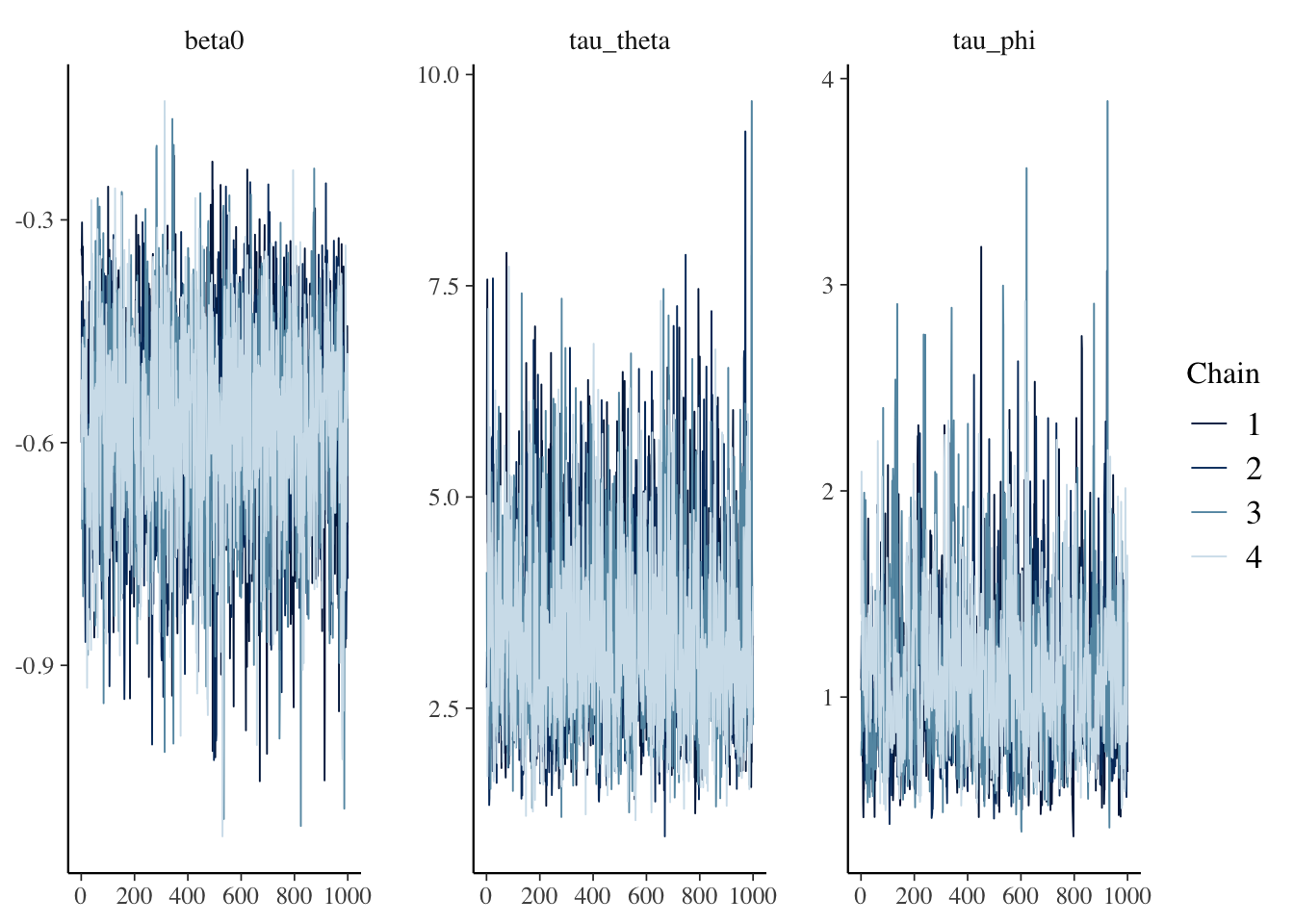
beta0とsigma_phi、sigma_thetaについて要約を表示します。
fit$summary(c("beta0", "sigma_phi", "sigma_theta"))
## # A tibble: 3 × 10
##   variable      mean median     sd    mad     q5    q95  rhat ess_bulk ess_tail
##   <chr>        <dbl>  <dbl>  <dbl>  <dbl>  <dbl>  <dbl> <dbl>    <dbl>    <dbl>
## 1 beta0       -0.582 -0.575 0.132  0.127  -0.805 -0.376  1.00    2102.    2333.
## 2 sigma_phi    1.00   0.990 0.166  0.163   0.756  1.29   1.01     873.    1663.
## 3 sigma_theta 0.569 0.562 0.0902 0.0897 0.431 0.731 1.00 1817. 2385.phiについて要約を表示します。
fit$summary(c("phi"))
## # A tibble: 200 × 10
##    variable    mean  median    sd   mad     q5   q95  rhat ess_bulk ess_tail
##    <chr>      <dbl>   <dbl> <dbl> <dbl>  <dbl> <dbl> <dbl>    <dbl>    <dbl>
##  1 phi[1]   -0.668  -0.653  0.816 0.823 -2.01  0.665  1.00    2693.    2751.
##  2 phi[2]   -0.378  -0.364  0.707 0.703 -1.55  0.767  1.00    2547.    2813.
##  3 phi[3]    0.179   0.203  0.628 0.627 -0.867 1.18   1.00    2213.    2938.
##  4 phi[4]    0.119   0.132  0.626 0.620 -0.924 1.12   1.00    2440.    2859.
##  5 phi[5]   -0.111  -0.0910 0.642 0.632 -1.19  0.932  1.00    2848.    2982.
##  6 phi[6]    0.0157  0.0130 0.626 0.630 -1.01  1.06   1.00    2723.    2815.
##  7 phi[7]    0.0229  0.0152 0.629 0.630 -0.997 1.03   1.00    2721.    2751.
##  8 phi[8]    0.327   0.329  0.603 0.597 -0.698 1.30   1.00    2708.    3163.
##  9 phi[9]    0.0833  0.0983 0.644 0.652 -0.969 1.12   1.00    2257.    2931.
## 10 phi[10]  -0.338  -0.322  0.786 0.790 -1.63  0.921  1.00    2562.    2859.
## # ℹ 190 more rows
thetaについて要約を表示します。
fit$summary(c("theta"))
## # A tibble: 200 × 10
## variable mean median sd mad q5 q95 rhat ess_bulk ess_tail
## <chr> <dbl> <dbl> <dbl> <dbl> <dbl> <dbl> <dbl> <dbl> <dbl>
## 1 theta[1] -0.224 -0.223 0.946 0.949 -1.78 1.31 1.00 5023. 3076.
## 2 theta[2] -0.251 -0.230 0.928 0.929 -1.76 1.26 1.00 4424. 3193.
## 3 theta[3] 0.509 0.500 0.892 0.920 -0.955 1.97 1.00 3819. 3059.
## 4 theta[4] 0.0887 0.102 0.901 0.907 -1.40 1.57 1.00 4246. 3479.
## 5 theta[5] -0.332 -0.325 0.956 0.951 -1.91 1.26 0.999 5005. 3113.
## 6 theta[6] 0.133 0.135 0.934 0.946 -1.48 1.68 1.00 4527. 2554.
## 7 theta[7] -0.349 -0.354 0.917 0.909 -1.88 1.17 1.00 4828. 2882.
## 8 theta[8] 0.436 0.452 0.904 0.908 -1.08 1.90 1.00 4435. 3342.
## 9 theta[9] 0.0903 0.0892 0.939 0.915 -1.47 1.65 1.00 4367. 2786.
## 10 theta[10] -0.273 -0.276 0.963 0.980 -1.84 1.29 1.00 4478. 2759.
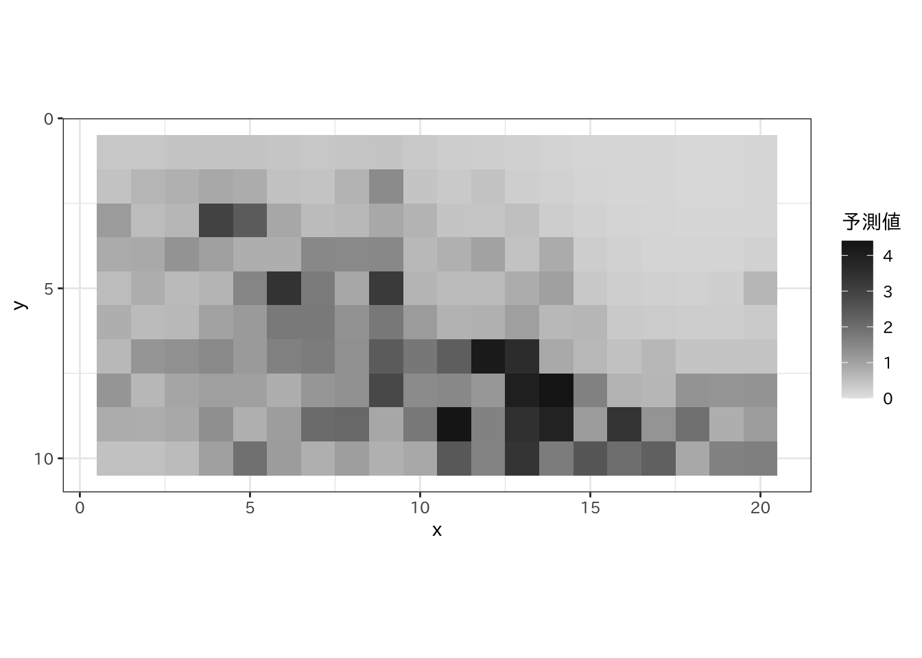
## # ℹ 190 more rows予測
各グリッドにおける株数の予測分布の平均値をプロットします。
fit$summary("mu") |>
  dplyr::mutate(x = rep(1:n.x, each = n.y),
                y = rep(1:n.y, n.x)) |>
  ggplot(aes(x = x, y = y)) +
  geom_tile(aes(fill = mean)) +
  scale_y_reverse(breaks = c(0, 5, 10)) +
  scale_fill_gradient(name = "予測値", limits = c(0, NA),
                      low = "grey90", high = "grey10") +
  coord_fixed(ratio = 1) +
  theme_bw(base_family = "IPAexGothic")