library(ggplot2)
library(betareg)
library(cmdstanr)
## This is cmdstanr version 0.5.2
## - CmdStanR documentation and vignettes: mc-stan.org/cmdstanr
## - CmdStan path: /usr/local/cmdstan
## - CmdStan version: 2.31.0
library(posterior)
## This is posterior version 1.3.1
##
##  次のパッケージを付け加えます: 'posterior'
##  以下のオブジェクトは 'package:stats' からマスクされています:
##
##     mad, sd, var
library(bayesplot)
## This is bayesplot version 1.10.0
## - Online documentation and vignettes at mc-stan.org/bayesplot
## - bayesplot theme set to bayesplot::theme_default()
##    * Does _not_ affect other ggplot2 plots
##    * See ?bayesplot_theme_set for details on theme setting
##
##  次のパッケージを付け加えます: 'bayesplot'
##  以下のオブジェクトは 'package:posterior' からマスクされています:
##
##     rhat
knitr::knit_engines$set(stan = cmdstanr::eng_cmdstan)(0, 1)の範囲をとるデータに対する回帰にはベータ回帰がよく使われます。Rのbetaregパッケージを使った場合とStanを使った場合、さらに単純に線形回帰を当てはめた場合を比較してみました。
準備
データ生成
以下のモデルで、ベータ分布に従うデータ\(Y\)を生成します。平均\(\mu\)をパラメータとして使う関係で、パラメータ\(\kappa\)も設定します。
\[ Y \sim \mathrm{Beta}(\alpha, \beta) \\ \mu = \frac{\alpha}{\alpha + \beta} = \mathrm{logit}^{-1}(-4.5 + 0.5 X) \\ \kappa = \alpha + \beta \]
set.seed(1234)
inv_logit <- function(x) {
  1 / (1 + exp(-x))
}
N <- 100
X <- runif(N, 0, 10)
logit_mu <- -4.5 + 0.7 * X
mu <-inv_logit(logit_mu)
kappa <- 6
alpha <- mu * kappa
beta <- (1 - mu) * kappa
Y <- rbeta(N, alpha, beta)
sim_data <- data.frame(X = X, Y = Y)
データ確認
データを図示します。
p0 <- ggplot(sim_data, aes(x = X, y = Y)) +
  geom_point()
print(p0)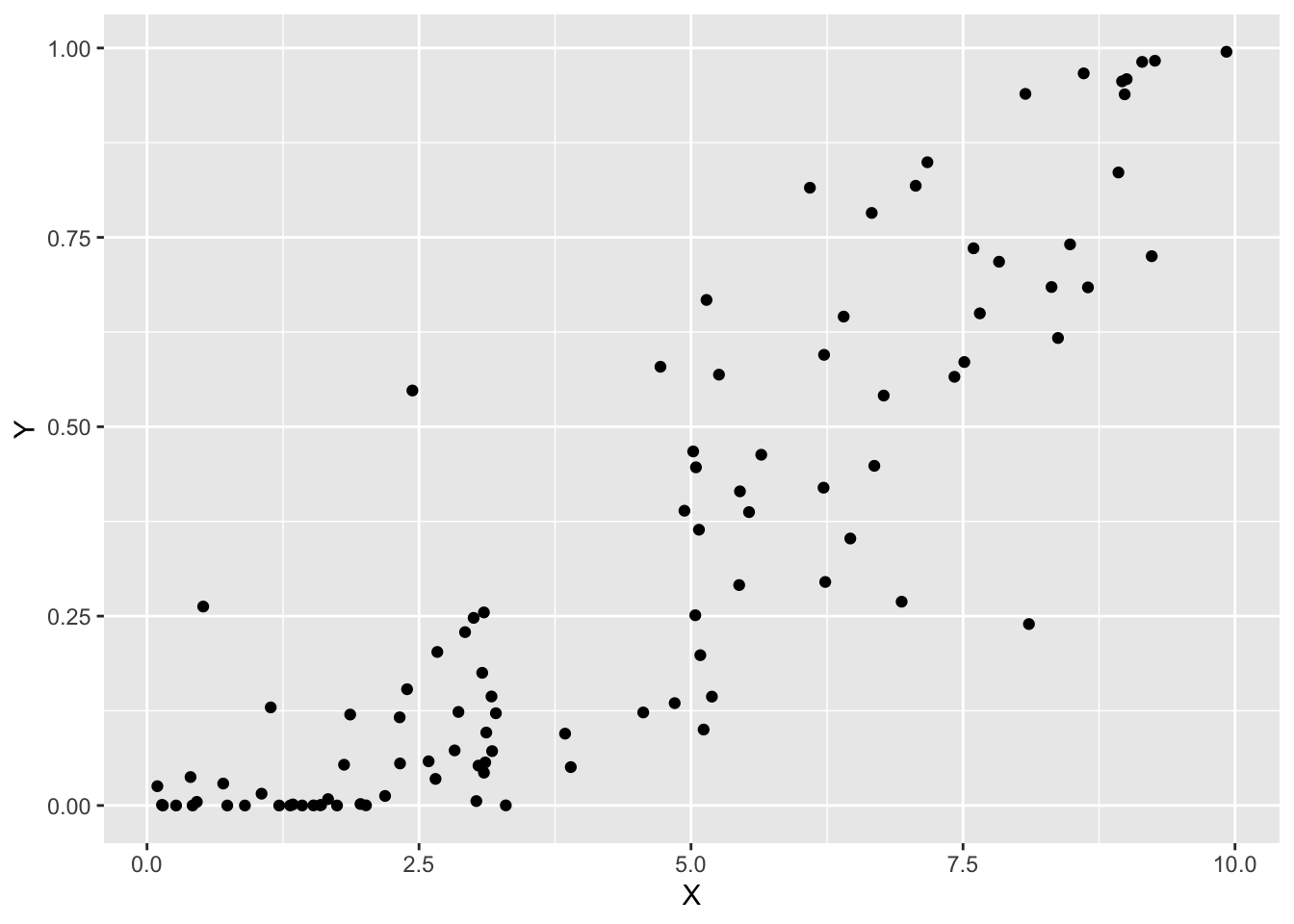
モデル
線形回帰
線形回帰を当てはめた場合です。
fit1 <- lm(Y ~ X, data = sim_data)
summary(fit1)
##
## Call:
## lm(formula = Y ~ X, data = sim_data)
##
## Residuals:
##      Min       1Q   Median       3Q      Max
## -0.46227 -0.08929 -0.00822  0.08569  0.42536
##
## Coefficients:
##              Estimate Std. Error t value Pr(>|t|)
## (Intercept) -0.126902   0.028096  -4.517 1.75e-05 ***
## X            0.102234   0.005424  18.848  < 2e-16 ***
## ---
## Signif. codes:  0 '***' 0.001 '**' 0.01 '*' 0.05 '.' 0.1 ' ' 1
##
## Residual standard error: 0.1504 on 98 degrees of freedom
## Multiple R-squared:  0.7838, Adjusted R-squared:  0.7816
## F-statistic: 355.2 on 1 and 98 DF,  p-value: < 2.2e-16
結果を図示します。
p0 +
  geom_abline(intercept = coef(fit1)[1],
              slope = coef(fit1)[2])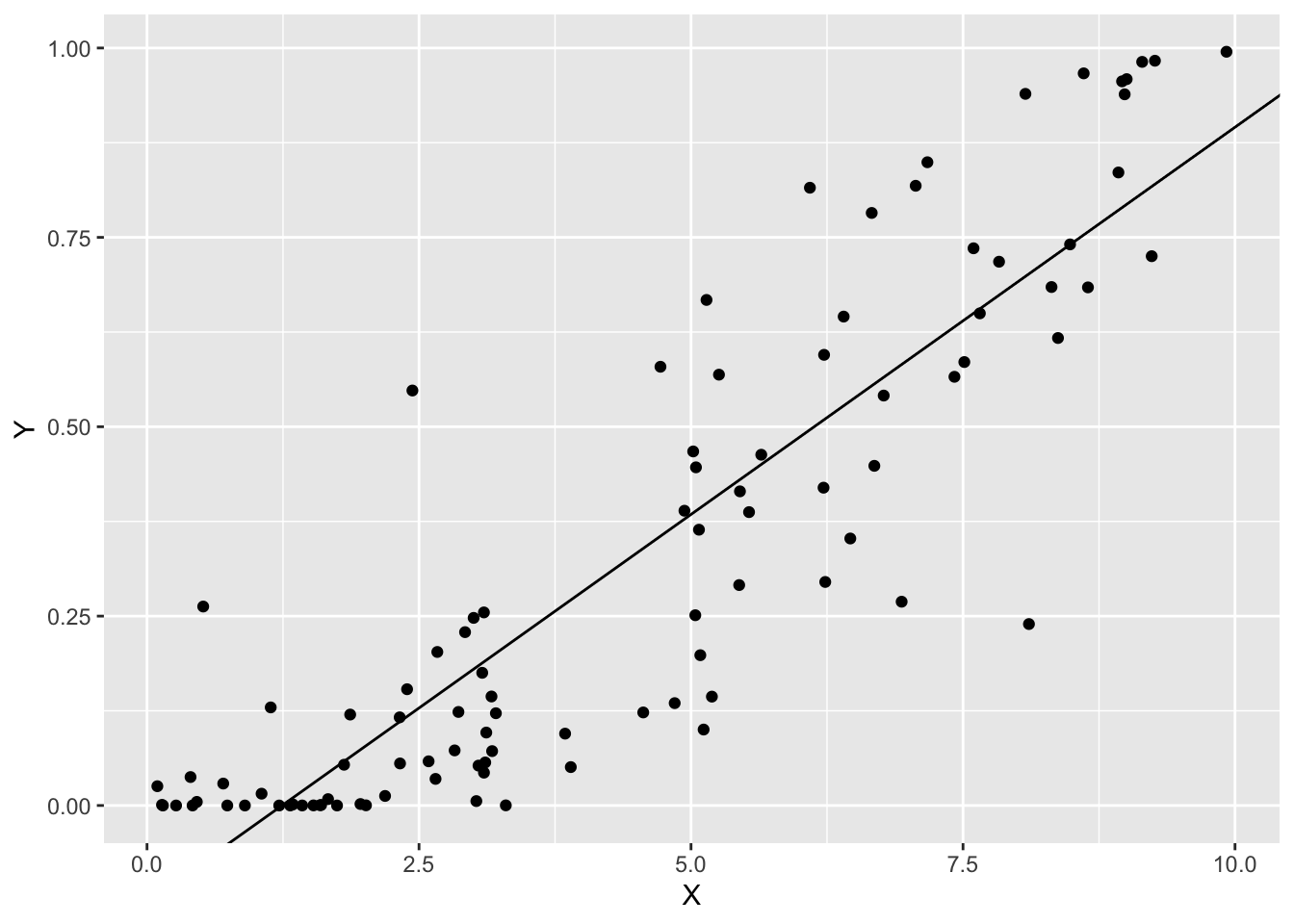
betaregパッケージを使ったベータ回帰
betaregパッケージを使った例です。
fit2 <- betareg(Y ~ X, sim_data, link = "logit")
summary(fit2)
##
## Call:
## betareg(formula = Y ~ X, data = sim_data, link = "logit")
##
## Standardized weighted residuals 2:
##     Min      1Q  Median      3Q     Max
## -3.0946 -0.5651  0.2074  0.7352  1.7862
##
## Coefficients (mean model with logit link):
##             Estimate Std. Error z value Pr(>|z|)
## (Intercept) -4.31787    0.24390  -17.70   <2e-16 ***
## X            0.68735    0.04227   16.26   <2e-16 ***
##
## Phi coefficients (precision model with identity link):
##       Estimate Std. Error z value Pr(>|z|)
## (phi)   5.6091     0.8828   6.354  2.1e-10 ***
## ---
## Signif. codes:  0 '***' 0.001 '**' 0.01 '*' 0.05 '.' 0.1 ' ' 1
##
## Type of estimator: ML (maximum likelihood)
## Log-likelihood: 259.4 on 3 Df
## Pseudo R-squared: 0.3637
## Number of iterations: 22 (BFGS) + 1 (Fisher scoring)
結果を図示します。
p0 +
  geom_function(fun = function(x)
    inv_logit(coef(fit2)[1] + coef(fit2)[2] * x))
Stanを使ったベータ回帰
Stanを使った例です。
Stanのコードは以下のようになります。
data {
  int<lower=0> N;               // number of data points
  vector[N] X;                  // explanatory variable
  vector<lower=0,upper=1>[N] Y; // objective variable
}

parameters {
  array[2] real beta;  // intercept and slope (logit scale)
  real<lower=0> kappa; // precision parameter
}

transformed parameters {
  vector<lower=0,upper=1>[N] mu = inv_logit(beta[1] + beta[2] * X);
}

model {
  Y ~ beta_proportion(mu, kappa);
  // priors
  beta ~ normal(0, 10);
}

generated quantities {
  vector<lower=0,upper=1>[N] yrep;

  for (n in 1:N)
    yrep[n] = beta_proportion_rng(mu[n], kappa);
}上のStanコードをコンパイルしたものをmodelというオブジェクトに格納して、サンプリングをおこないます。
stan_data <- list(N = N, X = X, Y = Y)
fit3 <- model$sample(data = stan_data,
                     iter_warmup = 1000, iter_sampling = 1000,
                     refresh = 1000)
## Running MCMC with 4 sequential chains...
##
## Chain 1 Iteration:    1 / 2000 [  0%]  (Warmup)
## Chain 1 Iteration: 1000 / 2000 [ 50%]  (Warmup)
## Chain 1 Iteration: 1001 / 2000 [ 50%]  (Sampling)
## Chain 1 Iteration: 2000 / 2000 [100%]  (Sampling)
## Chain 1 finished in 0.3 seconds.
## Chain 2 Iteration:    1 / 2000 [  0%]  (Warmup)
## Chain 2 Iteration: 1000 / 2000 [ 50%]  (Warmup)
## Chain 2 Iteration: 1001 / 2000 [ 50%]  (Sampling)
## Chain 2 Iteration: 2000 / 2000 [100%]  (Sampling)
## Chain 2 finished in 0.3 seconds.
## Chain 3 Iteration:    1 / 2000 [  0%]  (Warmup)
## Chain 3 Iteration: 1000 / 2000 [ 50%]  (Warmup)
## Chain 3 Iteration: 1001 / 2000 [ 50%]  (Sampling)
## Chain 3 Iteration: 2000 / 2000 [100%]  (Sampling)
## Chain 3 finished in 0.3 seconds.
## Chain 4 Iteration:    1 / 2000 [  0%]  (Warmup)
## Chain 4 Iteration: 1000 / 2000 [ 50%]  (Warmup)
## Chain 4 Iteration: 1001 / 2000 [ 50%]  (Sampling)
## Chain 4 Iteration: 2000 / 2000 [100%]  (Sampling)
## Chain 4 finished in 0.3 seconds.
##
## All 4 chains finished successfully.
## Mean chain execution time: 0.3 seconds.
## Total execution time: 1.3 seconds.
fit3$summary(variables = c("beta", "kappa"))
## # A tibble: 3 × 10
##   variable   mean median     sd    mad     q5    q95  rhat ess_bulk ess_tail
##   <chr>     <dbl>  <dbl>  <dbl>  <dbl>  <dbl>  <dbl> <dbl>    <dbl>    <dbl>
## 1 beta[1]  -4.33  -4.33  0.218  0.222  -4.69  -3.97   1.00    1172.    1550.
## 2 beta[2]   0.690  0.689 0.0388 0.0390  0.628  0.755  1.00    1162.    1561.
## 3 kappa     5.69   5.65  0.851  0.870   4.36   7.12   1.00    1560.    1739.
結果を図示します。
beta_mean <- fit3$summary("beta")$mean
p0 +
  geom_function(fun = function(x)
    inv_logit(beta_mean[1] + beta_mean[2] * x))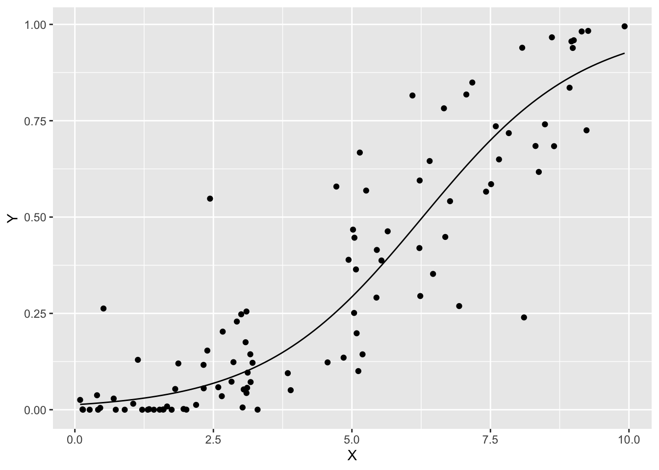
事後予測検査をしてみます。
yrep <- fit3$draws("yrep") |>
  as_draws_matrix()
ppc_dens_overlay(y = Y, yrep = yrep[1:100, ])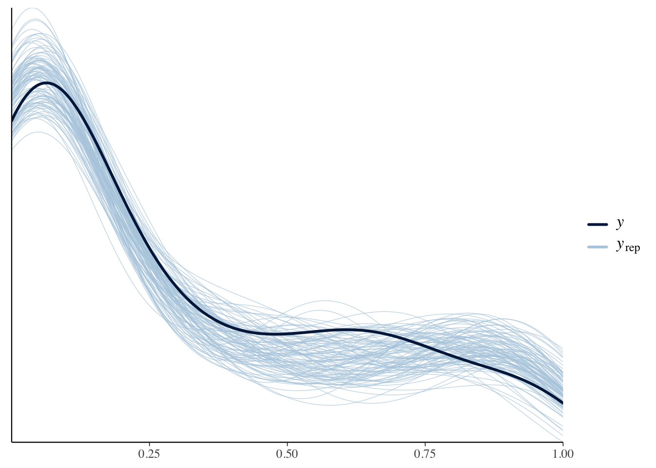
参考文献
- Imad Ali, Jonah Gabry and Ben Goodrich (2020) Modeling Rates/Proportions using Beta Regression with rstanarm. https://mc-stan.org/rstanarm/articles/betareg.html