library(ggplot2)
library(zoib)
##  要求されたパッケージ rjags をロード中です
##  要求されたパッケージ coda をロード中です
## Linked to JAGS 4.3.1
## Loaded modules: basemod,bugs
##  要求されたパッケージ Formula をロード中です
##  要求されたパッケージ abind をロード中です
library(cmdstanr)
## This is cmdstanr version 0.5.3
## - CmdStanR documentation and vignettes: mc-stan.org/cmdstanr
## - CmdStan path: /usr/local/cmdstan
## - CmdStan version: 2.31.0
library(posterior)
## This is posterior version 1.3.1
##
##  次のパッケージを付け加えます: 'posterior'
##  以下のオブジェクトは 'package:stats' からマスクされています:
##
##     mad, sd, var
library(bayesplot)
## This is bayesplot version 1.10.0
## - Online documentation and vignettes at mc-stan.org/bayesplot
## - bayesplot theme set to bayesplot::theme_default()
##    * Does _not_ affect other ggplot2 plots
##    * See ?bayesplot_theme_set for details on theme setting
##
##  次のパッケージを付け加えます: 'bayesplot'
##  以下のオブジェクトは 'package:posterior' からマスクされています:
##
##     rhat
knitr::knit_engines$set(stan = cmdstanr::eng_cmdstan)ベータ分布では、0(や1)そのものを含むデータは扱えません。0となる場合をモデルに組み込むことで0を扱えるようにします。
準備
モデル
\[z \sim \mathrm{Bern}(p)\] \[\mathrm{logit}(p) = \alpha_0 + \alpha_1 x\] \[y = 0 \quad \text{if} \, z = 0\] \[y \sim \mathrm{Beta}(\mu, \kappa) \quad \text{if} \, z = 1\] \[\mathrm{logit}(\mu) = \beta_0 + \beta_1 x\]
2値変数のzは確率pで1に、1-pで0になるとします。z=1のときは、目的変数yはベータ分布にしたがいますが、z=0のときはy=0となるとしています。
データ生成
模擬データを生成します。
set.seed(1234)
inv_logit <- function(x) {
  1 / (1 + exp(-x))
}
N <- 100
X <- runif(N, 0, 10)
p <- inv_logit(-4.5 + 2 * X)
mu <-inv_logit(-1 + 0.3 * X)
kappa <- 6
alpha <- mu * kappa
beta <- (1 - mu) * kappa
z <- rbinom(N, 1, p)
Y <- z * rbeta(N, alpha, beta)
sim_data <- data.frame(X = X, Y = Y)
データを確認します。
p0 <- ggplot(sim_data, aes(x = X, y = Y)) +
  geom_point()
print(p0)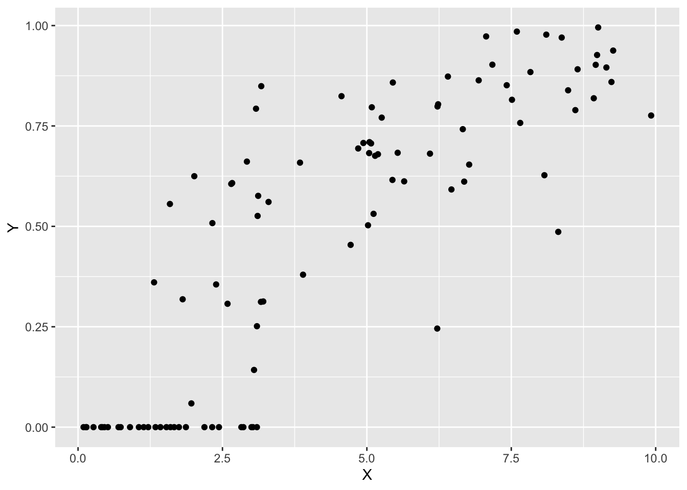
線形回帰
通常の線形回帰をあてはめると以下のようになります。
fit1 <- lm(Y ~ X, data = sim_data)
summary(fit1)
##
## Call:
## lm(formula = Y ~ X, data = sim_data)
##
## Residuals:
##      Min       1Q   Median       3Q      Max
## -0.42739 -0.13075 -0.03495  0.13098  0.50236
##
## Coefficients:
##             Estimate Std. Error t value Pr(>|t|)
## (Intercept) 0.007131   0.036579   0.195    0.846
## X           0.107071   0.007062  15.162   <2e-16 ***
## ---
## Signif. codes:  0 '***' 0.001 '**' 0.01 '*' 0.05 '.' 0.1 ' ' 1
##
## Residual standard error: 0.1958 on 98 degrees of freedom
## Multiple R-squared:  0.7011, Adjusted R-squared:  0.6981
## F-statistic: 229.9 on 1 and 98 DF,  p-value: < 2.2e-16
結果を図示します。
p0 +
  geom_abline(intercept = coef(fit1)[1],
              slope = coef(fit1)[2])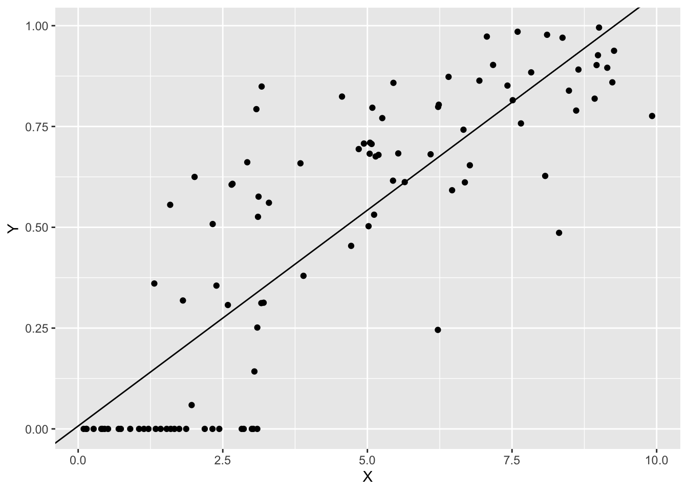
zoibパッケージを使用したゼロ過剰ベータ回帰
Rのzoibパッケージのzoib()関数を使ったゼロ過剰ベータ回帰です。
fit2 <- zoib(Y ~ X | 1 | X, data = sim_data,
zero.inflation = TRUE, one.inflation = FALSE,
n.chain = 3, n.iter = 10000, n.burn = 2000, n.thin = 8)
## [1] "***************************************************************************"
## [1] "* List of parameter for which the posterior samples are generated *"
## [1] "* b: regression coeff in the linear predictor for the mean of beta dist'n *"
## [1] "* d: regression coeff in the linear predictor for the sum of the two *"
## [1] "* shape parameters in the beta distribution *"
## [1] "* b0: regression coeff in the linear predictor for Prob(y=0) *"
## [1] "* b1: regression coeff in the linear predictor for Prob(y=1) *"
## [1] "***************************************************************************"
## Compiling model graph
## Resolving undeclared variables
## Allocating nodes
## Graph information:
## Observed stochastic nodes: 100
## Unobserved stochastic nodes: 18
## Total graph size: 4846
##
## Initializing model
##
## NOTE: Stopping adaptation
##
##
## [1] "NOTE: in the header of Markov Chain Monte Carlo (MCMC) output of"
## [1] "parameters (coeff), predicted values (ypred), residuals (resid), and"
## [1] "standardized residuals (resid.std), *Start, End, Thinning Interval*"
## [1] "values are after the initial burning and thinning periods specified"
## [1] "by the user. For example, n.iter = 151, n.thin = 2, n.burn=1,"
## [1] "then MCMC header of the *coeff* output would read as follows"
## [1] "-----------------------------------------"
## [1] "Markov Chain Monte Carlo (MCMC) output:"
## [1] "Start = 1"
## [1] "End = 75"
## [1] "Thinning interval = 1"
## [1] " "
## [1] " "
## [1] "Coefficients are presented in the order of b, "
## [1] "b0 (if zero.inflation=TRUE), b1 (if one.inflation=TRUE), and d"
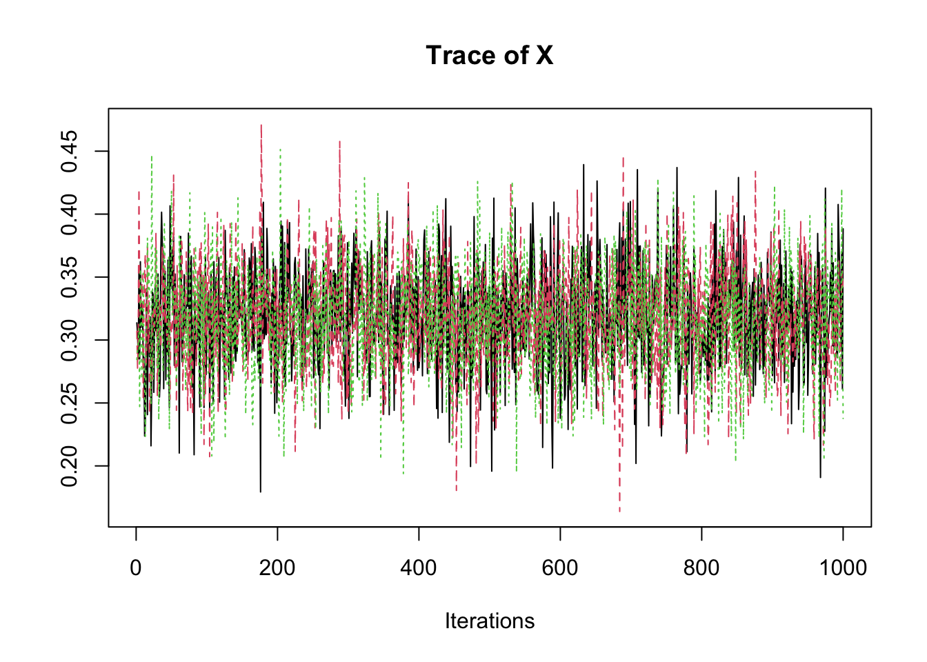
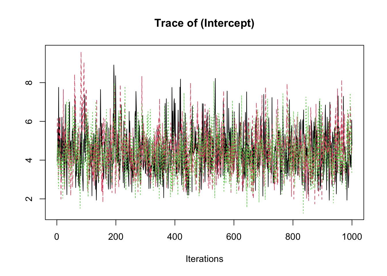
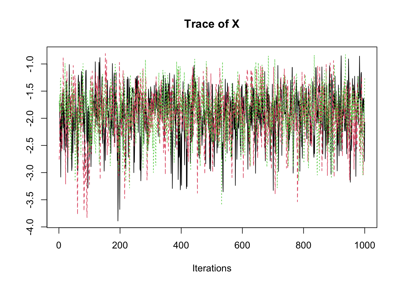
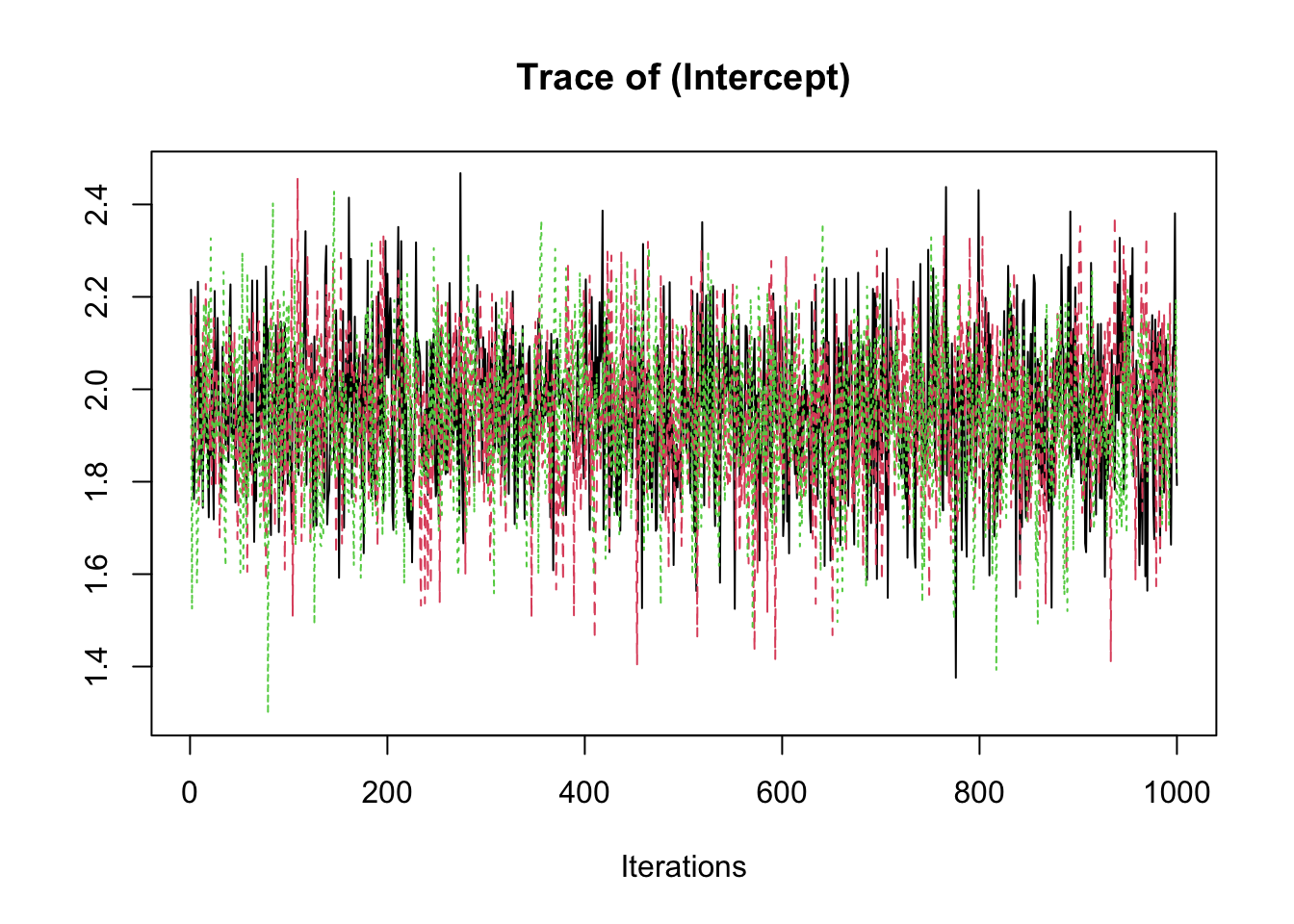
samp <- fit2$coeff
traceplot(samp)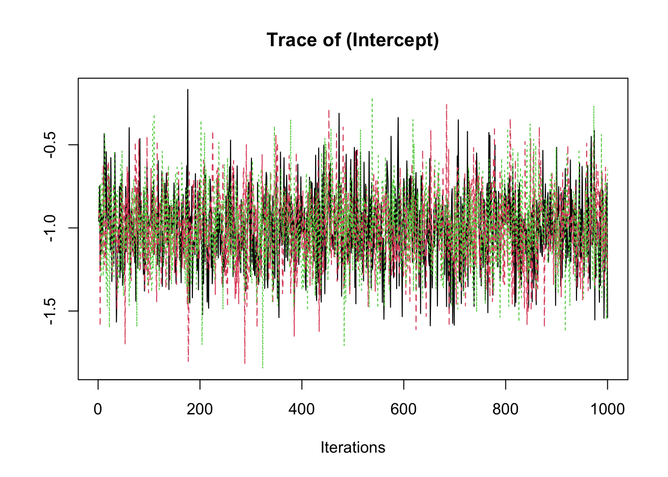
summary(samp)
##
## Iterations = 1:1000
## Thinning interval = 1
## Number of chains = 3
## Sample size per chain = 1000
##
## 1. Empirical mean and standard deviation for each variable,
##    plus standard error of the mean:
##
##                Mean      SD  Naive SE Time-series SE
## (Intercept) -1.0042 0.23186 0.0042332      0.0043135
## X            0.3178 0.04167 0.0007608      0.0007735
## (Intercept)  4.4267 1.13638 0.0207473      0.0283880
## X           -1.9283 0.46037 0.0084052      0.0124950
## (Intercept)  1.9480 0.16267 0.0029699      0.0029823
##
## 2. Quantiles for each variable:
##
##                2.5%     25%     50%     75%   97.5%
## (Intercept) -1.4564 -1.1626 -1.0026 -0.8486 -0.5361
## X            0.2337  0.2898  0.3182  0.3449  0.3990
## (Intercept)  2.4438  3.6069  4.3476  5.1219  6.9407
## X           -2.9743 -2.1989 -1.8915 -1.6098 -1.1338
## (Intercept)  1.6083  1.8433  1.9514  2.0578  2.2558
zoibは、内部でJAGSを使用しています。そのモデルコードを見てみます。
fit2$MCMC.model
## JAGS model:
##
## model
## {
##   K <-1000
##   for(i in 1:n)
##   {
##       d0[i]<- step(0.0001-y[i])    #d=1 if y=0
##
##       # 1: mean
##       logit(ph1[i,1])  <- inprod(b[], xmu.1[i,])
##       cloglog(ph1[i,2])<- inprod(b[], xmu.1[i,])
##       probit(ph1[i,3]) <- inprod(b[], xmu.1[i,])
##       mu[i] <- inprod(ph1[i, ],link[1,])
##
##       # 2: sum
##       log(den[i]) <- inprod(d[],  xsum.1[i,])
##
##       s[i,1]<- den[i]*mu[i]
##        s[i,2]<- den[i]*(1-mu[i])
##
##       # 3: zero
##       logit(ph2[i,1])  <- inprod(b0[], x0.1[i,])
##       cloglog(ph2[i,2])<- inprod(b0[], x0.1[i,])
##       probit(ph2[i,3]) <- inprod(b0[], x0.1[i,])
##       p0[i]<- inprod(ph2[i, ],link[2,])
##
##       ll[i]<- d0[i]*log(p0[i])+(1-d0[i])*log(1-p0[i])+
##               (1-d0[i])*((s[i,1]-1)*log(y[i])+(s[i,2]-1)*log(1-y[i])+
##                   loggam(s[i,1]+s[i,2])-loggam(s[i,1])-loggam(s[i,2]))
##       trick[i] <- K-ll[i]
##       zero[i] ~ dpois(trick[i])
##
##       ypred[i] <- (1-p0[i])*mu[i]
##   }
##
##   #################      regression coeff   ##################
##   tmp1 ~ dnorm(0, hyper[1,1])
##   b[1] <- tmp1
##   for(i in 1:(p.xmu-1))
##   {
##     ###   diffuse normal ###
##      b.tmp[i,1] ~ dnorm(0.0, hyper[1,2])
##
##     ###   L1 (lasso) ###
##      b.tmp[i,2] ~ dnorm(0.0,taub.L1[i]);
##     taub.L1[i] <- 1/sigmab.L1[i];
##     sigmab.L1[i] ~ dexp(hyper[1,3]);
##
##     ###   L2  (ridge) ###
##     b.tmp[i,3] ~ dnorm(0.0,taub.L2);
##
##      ###   ARD  ###
##      b.tmp[i,4] ~ dnorm(0.0,taub.ARD[i]);
##     taub.ARD[i] ~ dgamma(hyper[1,5], hyper[1,5]);
##
##     b[i+1] <- inprod(b.tmp[i, ],prior1[1,])
##      }
##   taub.L2 ~ dgamma(hyper[1,4],hyper[1,4]);  # L2 (ridge)
##
##
##   tmp2 ~ dnorm(0, hyper[2,1])
##   d[1] <- tmp2
##  for(i in 1:(p.xsum-1))
##  {
##      d.tmp[i,1] ~ dnorm(0, hyper[2,2])
##
##      d.tmp[i,2] ~ dnorm(0.0,taud.L1[i]);
##     taud.L1[i] <- 1/sigmad.L1[i];
##     sigmad.L1[i] ~ dexp(hyper[2,3]);
##
##     d.tmp[i,3] ~ dnorm(0.0,taud.L2);
##
##      d.tmp[i,4] ~ dnorm(0.0,taud.ARD[i]);
##     taud.ARD[i] ~ dgamma(hyper[2,5], hyper[2,5]);
##
##     d[i+1] <- inprod(d.tmp[i, ],prior1[2,])
##      }
##   taud.L2 ~ dgamma(hyper[2,4],hyper[2,4]);
##
##   tmp3~ dnorm(0, hyper[3,1])
##   b0[1] <- tmp3
##   for(i in 1:(p.x0-1))
##  {
##      b0.tmp[i,1] ~ dnorm(0, hyper[3,2])
##
##      b0.tmp[i,2] ~ dnorm(0.0,taub0.L1[i]);
##     taub0.L1[i] <- 1/sigmab0.L1[i];
##     sigmab0.L1[i] ~ dexp(hyper[3,3]);
##
##     b0.tmp[i,3] ~ dnorm(0.0,taub0.L2);
##
##      b0.tmp[i,4] ~ dnorm(0.0,taub0.ARD[i]);
##     taub0.ARD[i] ~ dgamma(hyper[3,5],hyper[3,5]);
##
##     b0[i+1] <- inprod(b0.tmp[i, ],prior1[3,])
##      }
##   taub0.L2 ~ dgamma(hyper[3,4],hyper[3,4]);
##
## }
##
## Fully observed variables:
##  hyper link n p.x0 p.xmu p.xsum prior1 x0.1 xmu.1 xsum.1 y zero
yが0.0001よりも小さい場合には、0として扱っているようです。
Stanを使用したゼロ過剰ベータ回帰
Stanのコードは以下のようになります。
data {
  int<lower=0> N;               // number of data points
  vector[N] X;                  // explanatory variable
  vector<lower=0,upper=1>[N] Y; // objective variable
  int<lower=0> N_xnew;          //
  vector[N_xnew] X_new;         // new x for prediction
}

parameters {
  array[2] real alpha; // intercept and slope in the probability model
                       // (logit scale)
  array[2] real beta;  // intercept and slope in the beta model
                       // (logit scale)
  real<lower=0> kappa; // precision parameter
}

transformed parameters {
  vector[N] logit_p = alpha[1] + alpha[2] * X;
  vector<lower=0,upper=1>[N] mu = inv_logit(beta[1] + beta[2] * X);
}

model {
  for (n in 1:N) {
    if (Y[n] == 0)
      target += bernoulli_logit_lpmf(0 | logit_p[n]);
    else
      target += bernoulli_logit_lpmf(1 | logit_p[n])
                  + beta_proportion_lpdf(Y[n] | mu[n], kappa);
  }

  // priors
  alpha ~ normal(0, 10);
  beta ~ normal(0, 10);
}

generated quantities {
  vector<lower=0,upper=1>[N] yrep; // replication for PPC
  vector<lower=0,upper=1>[N_xnew] ypred; // prediction for new X
  vector[N_xnew] new_logit_p = alpha[1] + alpha[2] * X_new;
  vector[N_xnew] new_mu = inv_logit(beta[1] + beta[2] * X_new);

  for (n in 1:N) {
    int z = bernoulli_logit_rng(logit_p[n]);
    yrep[n] = z * beta_proportion_rng(mu[n], kappa);
  }

  for (n in 1:N_xnew) {
    int z = bernoulli_logit_rng(new_logit_p[n]);
    ypred[n] = z * beta_proportion_rng(new_mu[n], kappa);
  }
}
cmdstanrを使用します。上のStanコードをコンパイルしたものをmodelオブジェクトに格納しておきます。
xnew <- seq(0, 10, length = 101)
stan_data <- list(N = N, X = X, Y = Y,
                  N_xnew = length(xnew), X_new = xnew)
fit3 <- model$sample(data = stan_data,
                     iter_warmup = 1000, iter_sampling = 3000,
                     refresh = 1000)
## Running MCMC with 4 sequential chains...
##
## Chain 1 Iteration:    1 / 4000 [  0%]  (Warmup)
## Chain 1 Iteration: 1000 / 4000 [ 25%]  (Warmup)
## Chain 1 Iteration: 1001 / 4000 [ 25%]  (Sampling)
## Chain 1 Iteration: 2000 / 4000 [ 50%]  (Sampling)
## Chain 1 Iteration: 3000 / 4000 [ 75%]  (Sampling)
## Chain 1 Iteration: 4000 / 4000 [100%]  (Sampling)
## Chain 1 finished in 2.1 seconds.
## Chain 2 Iteration:    1 / 4000 [  0%]  (Warmup)
## Chain 2 Iteration: 1000 / 4000 [ 25%]  (Warmup)
## Chain 2 Iteration: 1001 / 4000 [ 25%]  (Sampling)
## Chain 2 Iteration: 2000 / 4000 [ 50%]  (Sampling)
## Chain 2 Iteration: 3000 / 4000 [ 75%]  (Sampling)
## Chain 2 Iteration: 4000 / 4000 [100%]  (Sampling)
## Chain 2 finished in 1.9 seconds.
## Chain 3 Iteration:    1 / 4000 [  0%]  (Warmup)
## Chain 3 Iteration: 1000 / 4000 [ 25%]  (Warmup)
## Chain 3 Iteration: 1001 / 4000 [ 25%]  (Sampling)
## Chain 3 Iteration: 2000 / 4000 [ 50%]  (Sampling)
## Chain 3 Iteration: 3000 / 4000 [ 75%]  (Sampling)
## Chain 3 Iteration: 4000 / 4000 [100%]  (Sampling)
## Chain 3 finished in 2.0 seconds.
## Chain 4 Iteration:    1 / 4000 [  0%]  (Warmup)
## Chain 4 Iteration: 1000 / 4000 [ 25%]  (Warmup)
## Chain 4 Iteration: 1001 / 4000 [ 25%]  (Sampling)
## Chain 4 Iteration: 2000 / 4000 [ 50%]  (Sampling)
## Chain 4 Iteration: 3000 / 4000 [ 75%]  (Sampling)
## Chain 4 Iteration: 4000 / 4000 [100%]  (Sampling)
## Chain 4 finished in 2.1 seconds.
##
## All 4 chains finished successfully.
## Mean chain execution time: 2.0 seconds.
## Total execution time: 8.5 seconds.
fit3$print(variables = c("alpha", "beta", "kappa"), digits = 2)
##  variable  mean median   sd  mad    q5   q95 rhat ess_bulk ess_tail
##  alpha[1] -4.37  -4.28 1.11 1.10 -6.33 -2.72 1.00     5553     4818
##  alpha[2]  1.91   1.87 0.45 0.44  1.24  2.70 1.00     5452     4953
##  beta[1]  -1.01  -1.01 0.23 0.23 -1.40 -0.64 1.00     5543     6374
##  beta[2]   0.32   0.32 0.04 0.04  0.25  0.39 1.00     5539     6640
##  kappa     7.26   7.19 1.19 1.17  5.45  9.36 1.00     8798     6953
事後予測検査をしてみます。
yrep <- fit3$draws("yrep") |>
  as_draws_matrix()
ppc_dens_overlay(y = Y, yrep = yrep[1:100, ])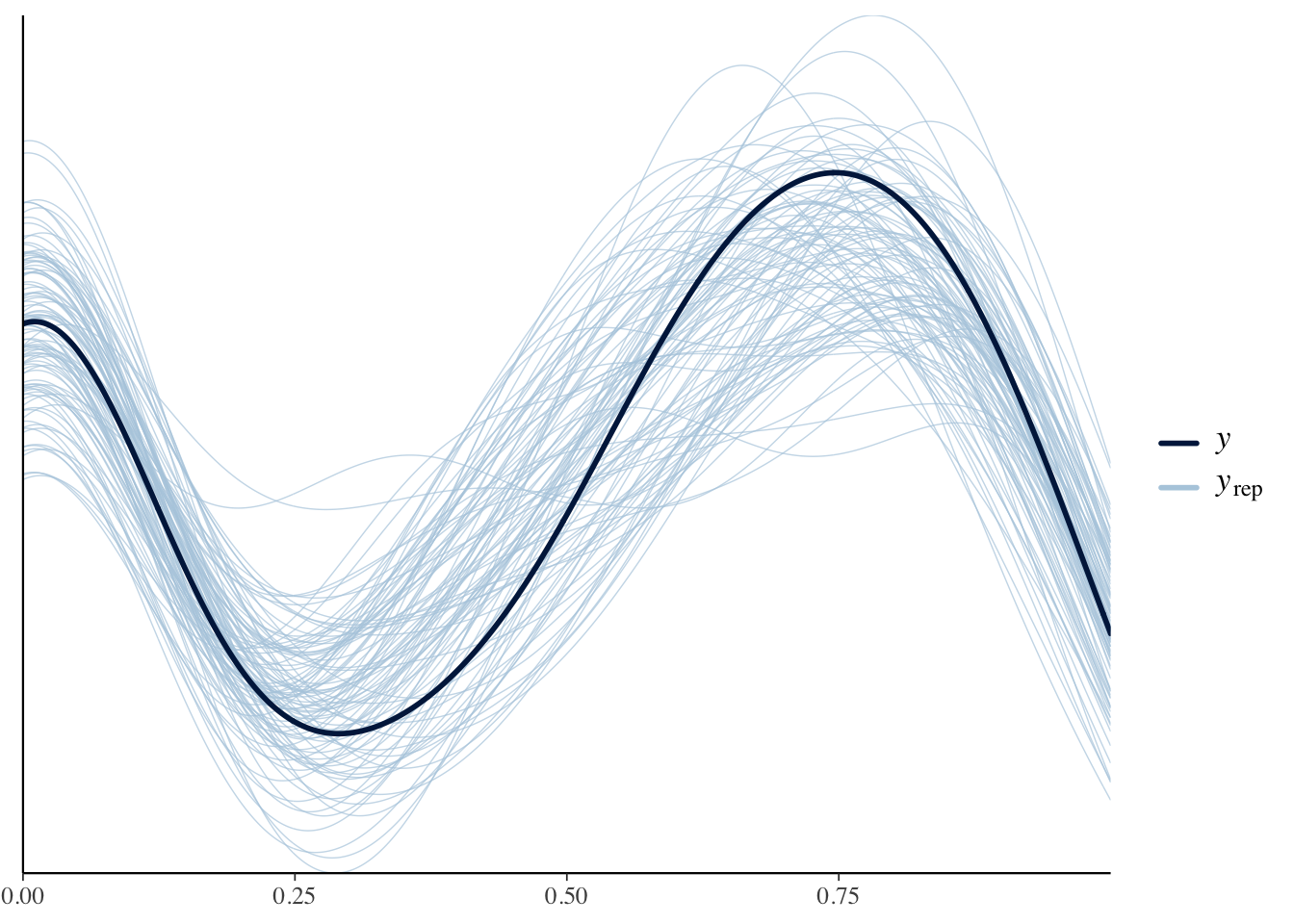
だいたいあっているようです。
説明変数Xに対して、z=1となる確率pと、ベータ分布の平均muの事後平均をプロットします。
x <- seq(0, 10, length = 101)
alpha <- fit3$summary("alpha")$mean
beta <- fit3$summary("beta")$mean
p <- inv_logit(alpha[1] + alpha[2] * x)
mu <- inv_logit(beta[1] + beta[2] * x)
df <- data.frame(X = x, p = p, mu = mu)
xとpの関係
ggplot(df, aes(x = X, y = p)) +
  geom_line() +
  ylim(0, 1)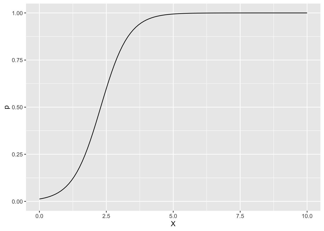
xとmuの関係
ggplot(df, aes(x = X, y = mu)) +
  geom_line() +
  ylim(0, 1)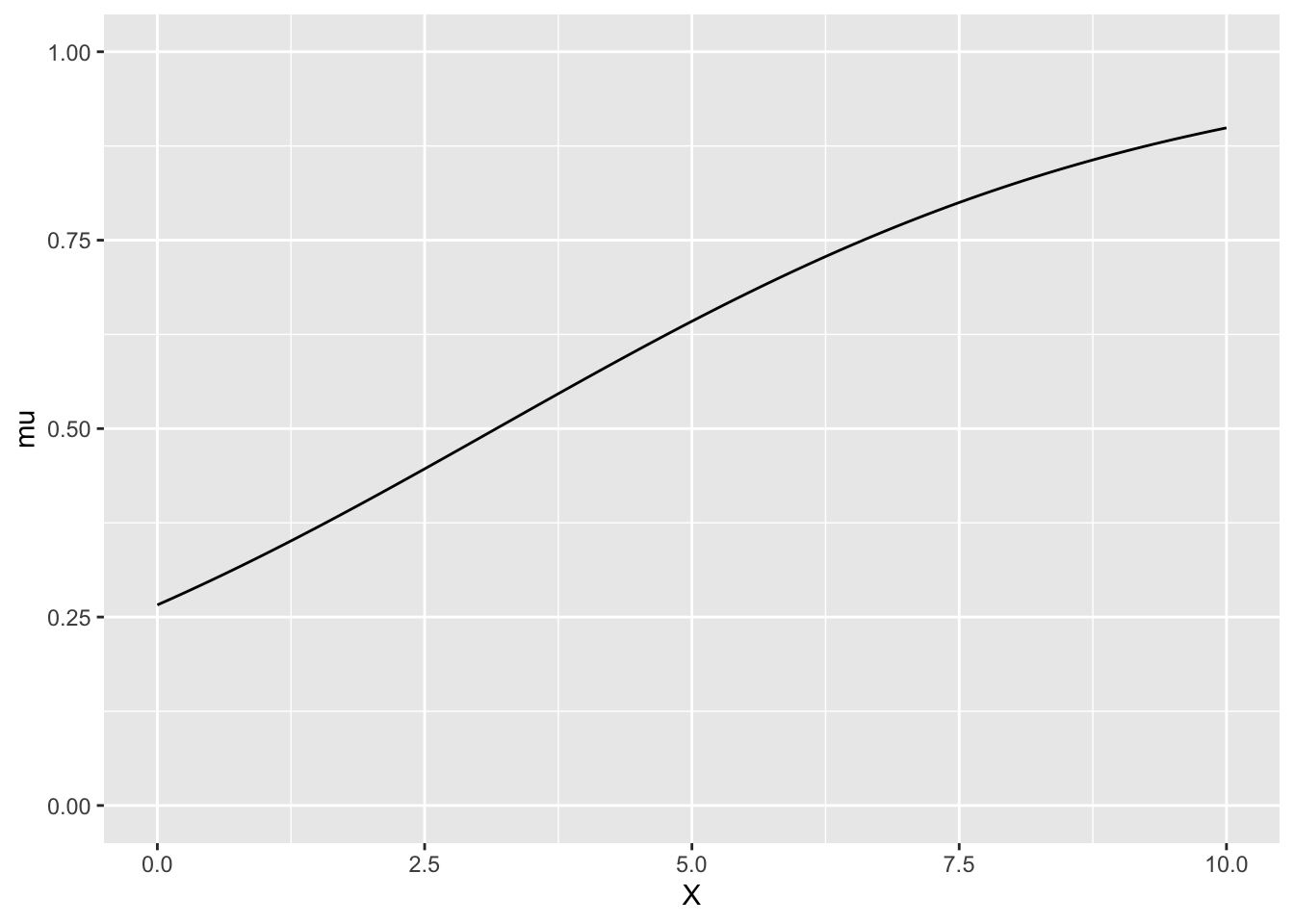
MCMCのサンプルを利用して、XとYの予測値(事後中央値と90%信用区間)との関係を、データの上にプロットします。
ypred <-  fit3$summary("ypred")
ggplot() +
  geom_ribbon(data = data.frame(x = xnew,
                                ymin = ypred$q5, ymax = ypred$q95),
              mapping = aes(x = x, ymin = ymin, ymax = ymax),
              alpha = 0.5) +
  geom_line(data = data.frame(x = xnew, y = ypred$median),
            mapping = aes(x = x, y = y)) +
  geom_point(data = sim_data, mapping = aes(x = X, y = Y))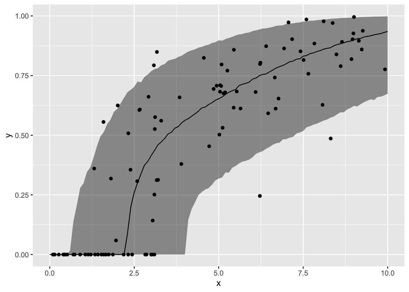
  ylim(0, 1)
## <ScaleContinuousPosition>
##  Range:
##  Limits:    0 --    1