library(ggplot2)
library(cmdstanr)
## This is cmdstanr version 0.5.3
## - CmdStanR documentation and vignettes: mc-stan.org/cmdstanr
## - CmdStan path: /usr/local/cmdstan
## - CmdStan version: 2.31.0
knitr::knit_engines$set(stan = cmdstanr::eng_cmdstan)

## Lotka-Volterra competitive equation
lv_fun <- function(x, r, K, alpha) {
  dx1_dt <- r[1] * x[1] * (1 - (x[1] + alpha[1] * x[2]) / K[1])
  dx2_dt <- r[2] * x[2] * (1 - (x[2] + alpha[2] * x[1]) / K[2])
  new_x1 <- max(0, x[1] + dx1_dt)
  new_x2 <- max(0, x[2] + dx2_dt)
  c(new_x1, new_x2)
}

## function to plot two curves
plot_lv <- function(r, K, alpha, init1 = c(1, 5), init2 = c(5, 1),
                    Nt = 50, name = rep(c("1", "2"), each = Nt),
                    max_axis = 30) {
  x <- matrix(0, ncol = 2, nrow = Nt * 2)
  x[1, ] <- init1
  for (t in 2:Nt) {
    x[t, ] <- lv_fun(x = x[t - 1, ], r = c(r1, r2),
                     K = c(K1, K2), alpha = c(alpha12, alpha21))
  }
  x[Nt + 1, ] <- init2
  for (t in (Nt + 2):(Nt * 2)) {
    x[t, ] <- lv_fun(x = x[t - 1, ], r = c(r1, r2),
                     K = c(K1, K2), alpha = c(alpha12, alpha21))
  }

  ggplot(data.frame(name, x)) +
    geom_path(aes(x = X1, y = X2, colour = name), linewidth = 1) +
    geom_point(aes(x = X1[1], y = X2[1]), colour = 2) +
    geom_point(aes(x = X1[Nt + 1], y = X2[Nt + 1]), colour = 3) +
    geom_segment(aes(x = K1, y = 0, xend = 0, yend = K1 / alpha12),
                 linewidth = 0.2, colour = "blue") +
    geom_segment(aes(x = 0, y = K2, xend = K2 / alpha21, yend = 0),
                 linewidth = 0.2, colour = "purple") +
    xlim(0, max_axis) + ylim(0, max_axis) +
    labs(x = "x1", y = "x2") +
    coord_fixed() +
    theme_bw() +
    theme(legend.position = "none")
}Stanの組み込み関数には、常微分方程式を解く関数があります。これを使った例として、ロトカ・ヴォルテラの競争方程式を組み込んだモデルのパラメーター推定をやってみます。
ロトカ・ヴォルテラの競争方程式
詳細は上のリンク先を見ていただきたいのですが、2種の生物からなる系をモデル化したものです。種1の個体数量x1と、種2の個体数量x2が、以下のような連立常微分方程式で定義されます。
\[\frac{dx_1}{dt} = r_1 x_1 \left[1 - \left(\frac{x_1 + \alpha_{12} x_2}{K_1}\right)\right]\] \[\frac{dx_2}{dt} = r_2 x_2 \left[1 - \left(\frac{x_2 + \alpha_{21} x_1}{K_2}\right)\right]\]
環境収容力K1, K2と、競争係数α12, α21の値により、個体数量(実数)の組み合わせ(x1, x2)の安定平衡点のパターンが4種類できます。 r1, r2 はそれぞれの種の内的自然増加率です。
Rによるシミュレーション
まずは、ライブラリの読み込みと、ロトカ・ヴォルテラの競争方程式の関数、グラフ表示の関数の定義です。競争方程式は、差分方程式で実装しています。
Example 1
K2 < K1 / α12 かつ K1 > K2 / α21 のとき:
青線と、紫線はアイソクライン直線、赤線と緑線は初期値(点)から安定平衡点にいたるまでの軌跡です(以下同様)。
Nt <- 100
r1 <- 0.3
r2 <- 0.4
K1 <- 25
K2 <- 15
alpha12 <- 0.95
alpha21 <- 0.95

plot_lv(r = c(r1, r2), K = c(K1, K2), alpha = c(alpha12, alpha21),
        Nt = Nt)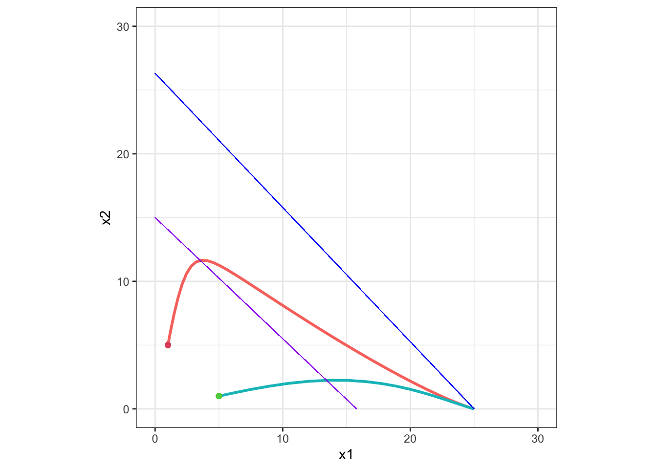
この場合、安定平衡点は x1 = K1, x2 = 0 です。
Example 2
K2 > K1 / α12 かつ K1 < K2 / α21 のとき:
Nt <- 100
r1 <- 0.3
r2 <- 0.4
K1 <- 15
K2 <- 25
alpha12 <- 0.95
alpha21 <- 0.95

plot_lv(r = c(r1, r2), K = c(K1, K2), alpha = c(alpha12, alpha21),
        Nt = Nt)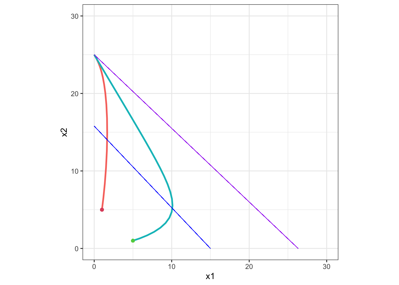
この場合、安定平衡点は x1 = 0, x2 = K2 です。
Example 3
K2 > K1 / α12 かつ K1 > K2 / α21 のとき:
Nt <- 100
r1 <- 0.3
r2 <- 0.4
K1 <- 25
K2 <- 25
alpha12 <- 1.2
alpha21 <- 1.5

plot_lv(r = c(r1, r2), K = c(K1, K2), alpha = c(alpha12, alpha21),
        Nt = Nt)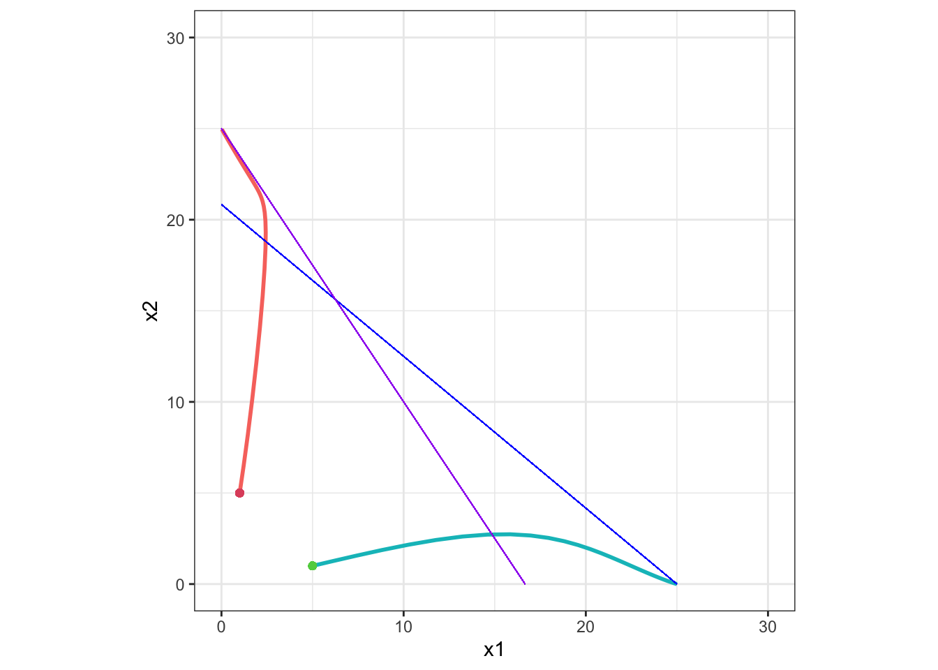
この場合、安定平衡点は、初期値により x1 = K1, x2 = 0 または x1 = 0, x2 = K2 となります。
Example 4
K2 < K1 / α12 かつ K1 < K2 / α21 のとき:
Nt <- 100
r1 <- 0.3
r2 <- 0.4
K1 <- 15
K2 <- 20
alpha12 <- 0.6
alpha21 <- 0.9

plot_lv(r = c(r1, r2), K = c(K1, K2), alpha = c(alpha12, alpha21),
                Nt = Nt)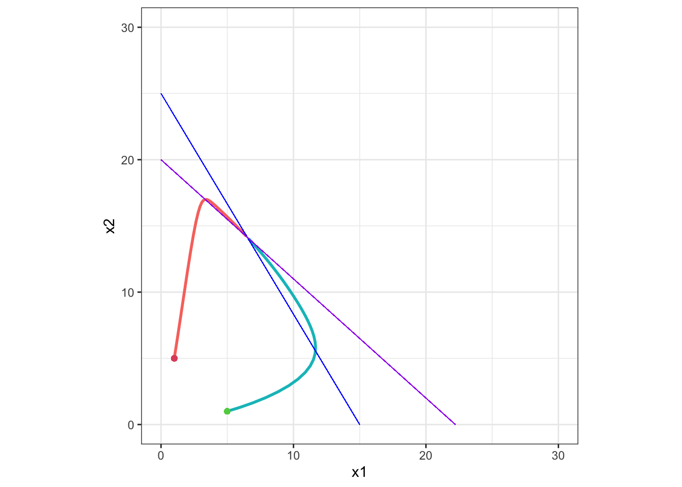
この場合、安定平衡点は x1 = (K1 - α12K2) / (1 - α12α21), x2 = (K2 - α21K1) / (1 - α12α21) となります。
Stanによるあてはめの例
両種の個体数量の軌跡がとれているときに、環境収容力と競争係数、内的自然増加率ほかをパラメーターとして推定します。
模擬データの生成
だいたい Example 4 に似たデータを生成しますが、ランダムなノイズが加わるようになっています。
set.seed(1234)

r1 <- 0.3
r2 <- 0.4
K1 <- 15
K2 <- 20
alpha12 <- 0.4
alpha21 <- 0.9
Nt <- 25

init1 <- c(3, 1)
x <- matrix(0, ncol = 2, nrow = Nt)
x[1, ] <- init1
for (t in 2:Nt) {
  x[t, ] <- lv_fun(x = x[t - 1, ], r = c(r1, r2),
                   K = c(K1, K2), alpha = c(alpha12, alpha21))
}
for (k in 1:2) {
  x[, k] <- rlnorm(Nt, log(x[, k]), 0.01)
}

p <- ggplot(data.frame(x1 = x[, 1], x2 = x[, 2])) +
  geom_point(aes(x = x1, y = x2)) +
  xlim(0, 15) + ylim(0, 15) +
  coord_fixed() +
  theme_bw()
print(p)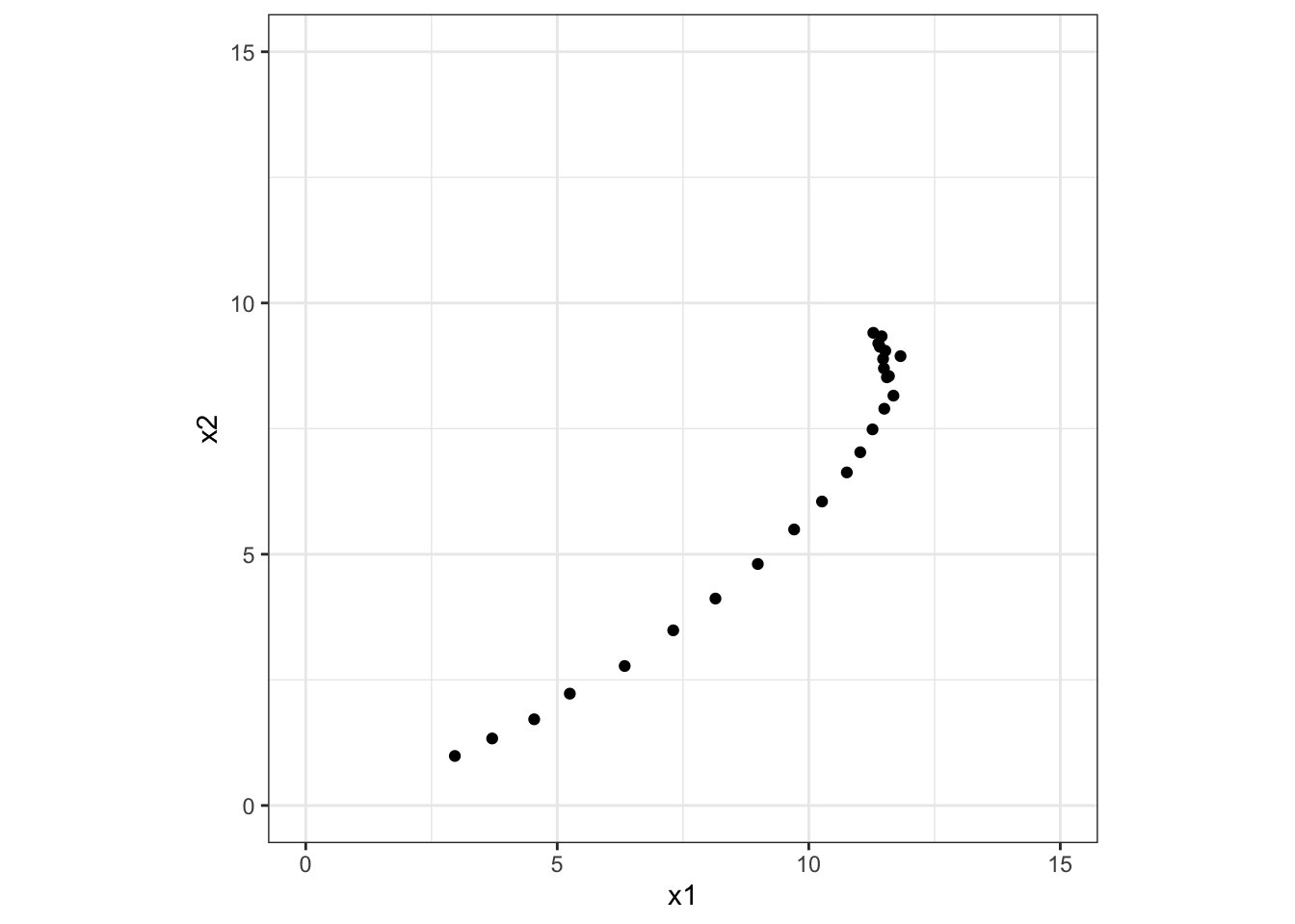
Stanのモデル
Stanのモデルです。ode_rk45が、ルンゲ・クッタ法により常微分方程式を解く関数です。
functions {
  vector dz_dt(real t, vector x, array[] real theta) {
    array[2] real r = theta[1:2];
    array[2] real K = theta[3:4];
    array[2] real alpha = theta[5:6];
    real dx1_dt = r[1] * x[1] * (1 - (x[1] + alpha[1] * x[2]) / K[1]);
    real dx2_dt = r[2] * x[2] * (1 - (x[2] + alpha[2] * x[1]) / K[2]);
    return [ dx1_dt, dx2_dt ]';
  }
}

data  {
  int<lower=0> N; // number of measurement times
  array[N] real ts; // measurement times > 0
  array[2] real<lower=0> y_init; // initial measured populations
  array[N, 2] real<lower=0> y; // measured populations
}

parameters {
  array[2] real<lower=0> r;
  array[2] real<lower=0> K;
  array[2] real<lower=0> alpha;
  vector<lower=0>[2] z_init; // initial population
  array[2] real<lower=0> sigma; // measurement errors
}

transformed parameters {
  array[6] real theta;
  theta[1:2] = r;
  theta[3:4] = K;
  theta[5:6] = alpha;
  array[N] vector<lower=0>[2] z = ode_rk45(dz_dt, z_init, 0, ts, theta);
}

model {
  r ~ normal(0, 2.5);
  K ~ normal(10, 5);
  alpha ~ normal(1, 1);
  sigma ~ normal(0, 2.5);
  z_init ~ lognormal(1, 2);
  for (k in 1:2) {
    y_init[k] ~ lognormal(log(z_init[k]), sigma[k]);
    y[ : , k] ~ lognormal(log(z[ : , k]), sigma[k]);
  }
}
あてはめ
cmdstanrを使用します。上のStanコードをコンパイルしたものをmodelオブジェクトに格納しておきます。
stan_data <- list(N = Nt - 1, ts = 1:(Nt - 1),
                  y_init = x[1, ], y = x[2:Nt, ])
fit <- model$sample(data = stan_data,
                    chains = 4, parallel_chains = 4,
                    iter_warmup = 2000, iter_sampling = 2000,
                    refresh = 2000)
## Running MCMC with 4 parallel chains...
##
## Chain 3 Iteration:    1 / 4000 [  0%]  (Warmup)
## Chain 4 Iteration:    1 / 4000 [  0%]  (Warmup)
## Chain 2 Iteration:    1 / 4000 [  0%]  (Warmup)
## Chain 1 Iteration:    1 / 4000 [  0%]  (Warmup)
## Chain 3 Iteration: 2000 / 4000 [ 50%]  (Warmup)
## Chain 3 Iteration: 2001 / 4000 [ 50%]  (Sampling)
## Chain 4 Iteration: 2000 / 4000 [ 50%]  (Warmup)
## Chain 4 Iteration: 2001 / 4000 [ 50%]  (Sampling)
## Chain 2 Iteration: 2000 / 4000 [ 50%]  (Warmup)
## Chain 2 Iteration: 2001 / 4000 [ 50%]  (Sampling)
## Chain 1 Iteration: 2000 / 4000 [ 50%]  (Warmup)
## Chain 1 Iteration: 2001 / 4000 [ 50%]  (Sampling)
## Chain 4 Iteration: 4000 / 4000 [100%]  (Sampling)
## Chain 4 finished in 129.1 seconds.
## Chain 3 Iteration: 4000 / 4000 [100%]  (Sampling)
## Chain 3 finished in 139.2 seconds.
## Chain 2 Iteration: 4000 / 4000 [100%]  (Sampling)
## Chain 2 finished in 136.2 seconds.
## Chain 1 Iteration: 4000 / 4000 [100%]  (Sampling)
## Chain 1 finished in 158.6 seconds.
##
## All 4 chains finished successfully.
## Mean chain execution time: 140.8 seconds.
## Total execution time: 171.7 seconds.
結果の要約です。
fit$summary(variables = c("r", "K", "alpha", "sigma"))
## # A tibble: 8 × 10
## variable mean median sd mad q5 q95 rhat ess_b…¹ ess_t…²
## <chr> <dbl> <dbl> <dbl> <dbl> <dbl> <dbl> <dbl> <dbl> <dbl>
## 1 r[1] 2.80e-1 2.80e-1 0.00557 0.00543 2.71e-1 0.289 1.00 2777. 3754.
## 2 r[2] 3.52e-1 3.53e-1 0.00498 0.00483 3.44e-1 0.361 1.00 2233. 3427.
## 3 K[1] 1.82e+1 1.81e+1 1.12 1.08 1.64e+1 20.2 1.00 2840. 3938.
## 4 K[2] 1.45e+1 1.44e+1 0.800 0.772 1.32e+1 15.8 1.00 2164. 3332.
## 5 alpha[1] 7.63e-1 7.57e-1 0.132 0.128 5.58e-1 0.994 1.00 2858. 3959.
## 6 alpha[2] 4.35e-1 4.31e-1 0.0652 0.0629 3.32e-1 0.546 1.00 2144. 3230.
## 7 sigma[1] 1.01e-2 9.86e-3 0.00163 0.00154 7.81e-3 0.0130 1.00 5010. 5056.
## 8 sigma[2] 8.27e-3 8.10e-3 0.00140 0.00130 6.36e-3 0.0108 1.00 5079. 3828.
## # … with abbreviated variable names ¹ess_bulk, ²ess_tailパラメーターの推定値は、設定した値とだいたいあっています。模擬データは差分方程式で生成しているので、多少ずれるかもしれません。
Stanでパラメーターと同時に推定した、ノイズなしの両種の個体数量の値を軌跡として元のグラフに重ねてみます。
z_mean <- rbind(fit$summary(variables = c("z_init"))$mean,
                matrix(fit$summary(variables = c("z"))$mean, ncol = 2))
p +
  geom_path(data = data.frame(z_mean),
            mapping = aes(x = X1, y = X2),
            colour = "red")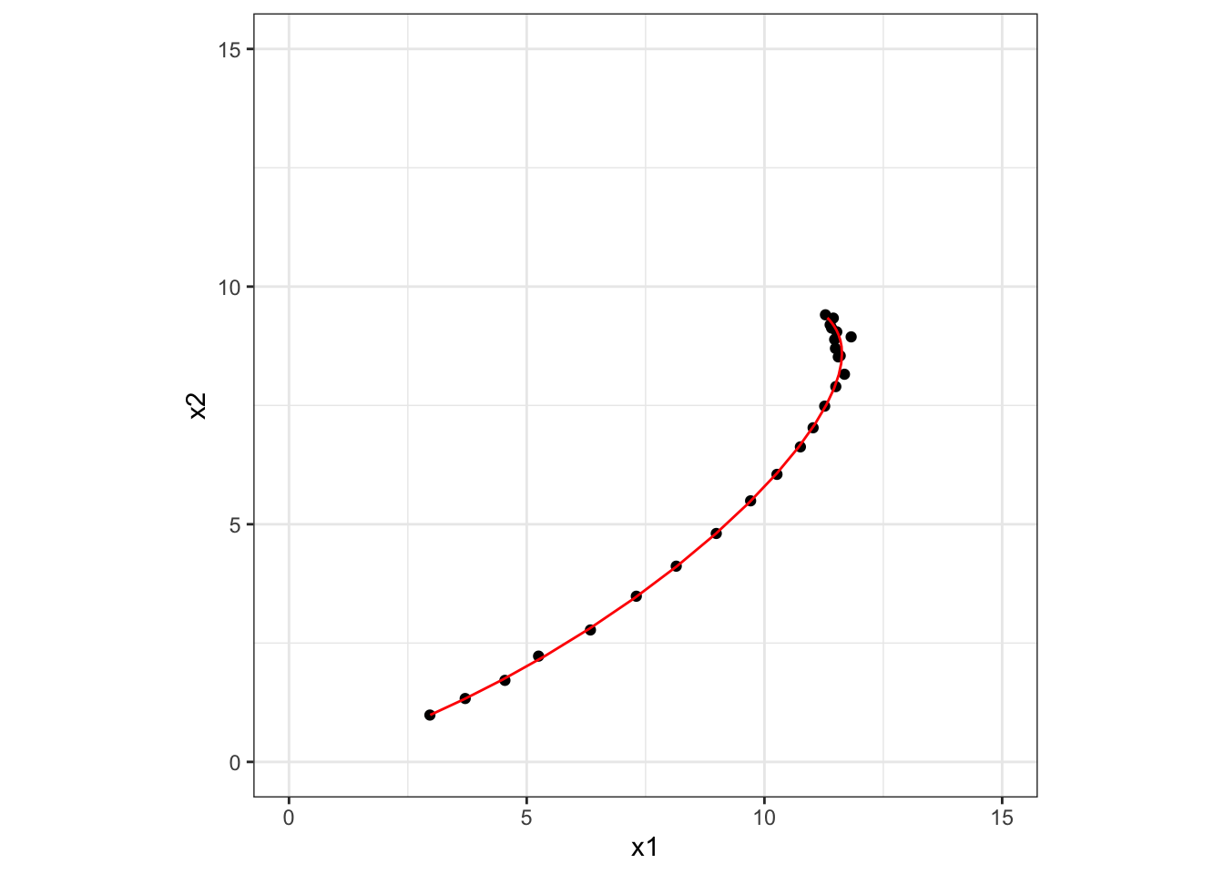
参考文献
- Bob Carpenter (2018) Predator-Prey Population Dynamics: the Lotka-Volterra model in Stan. https://mc-stan.org/users/documentation/case-studies/lotka-volterra-predator-prey.html