library(cmdstanr)
## This is cmdstanr version 0.5.3
## - CmdStanR documentation and vignettes: mc-stan.org/cmdstanr
## - CmdStan path: /usr/local/cmdstan
## - CmdStan version: 2.32.2
knitr::knit_engines$set(stan = cmdstanr::eng_cmdstan)
set.seed(1)Stanで、『生態学のための階層モデリング』8.3節にある標準距離標本抽出法モデルの解析をやってみます。
準備
CmdStanRを使用します。
標準距離標本抽出法
詳細は前掲書をご覧いただきたいのですが、観測者やトランセクトからの距離に応じて検出確率が変化するという観測過程により、生物の個体数を推定するというものです。
模擬データの生成
中心から両側に一定幅の調査範囲があるベルトトランセクトを想定して模擬データを生成します。
まず、検出確率の関数として半正規検出関数を定義します。
## Half-normal detection function
g <- function(x, sigma) {
  exp(-x^2 / (2 * sigma^2))
}
実際の個体数として N (=250) 個体、半正規検出関数の尺度パラメータとして sigma (=30)、トランセクトの片側の幅として width (=100) を与えます。
N <- 250     # Number of individuals
sigma <- 30  # Scale parameter of half-normal detection function
width <- 100 # Half-width of the transect
各個体は一様分布するとして距離データ xall を生成します。そこから距離に応じた検出確率 p で発見されたものだけを x に残します。
xall <- runif(N, -width, width) # Distance
p <- g(xall, sigma)             # Detection probability
y <- rbinom(N, 1, p)            # Detection
x <- abs(xall[y == 1])          # Distance to detected individuals
データの確認
観測された個体数です。
length(x)
## [1] 101
観測個体までの距離をヒストグラムで示します。
hist(x)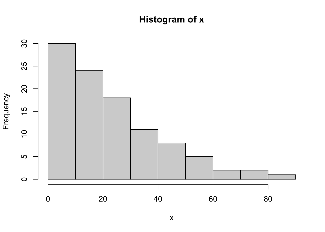
Stanのモデル
データ拡大法により、実際の個体数を推定するモデルとなっています。パラメータのomegaは、観測個体数+追加データ数のうち実際に存在する割合(データ拡大パラメータ)です。同じくx_augは、追加データの(観測されていない)距離データです。
data {
  int<lower=0> N_obs; // Number of observed individuals
  int<lower=0> N_aug; // Number of augmentated zeros
  real<lower=0> B;    // Transect width
  vector<lower=0, upper=B>[N_obs] X; // Distance data
}

parameters {
  real<lower=0, upper=100> sigma;  // Scale parameter of detection func.
  real<lower=0, upper=1> omega;    // Inclusion parameter
  vector<lower=0, upper=B>[N_aug] x_aug; // Unobserved distance data
}

transformed parameters {
  vector[N_obs + N_aug] p; // Detection probability

  // Observed data
  for (i in 1:N_obs)
    p[i] = exp(-X[i]^2 / (2 * sigma^2));

  // Augumented zero data
  for (i in (N_obs + 1):(N_obs + N_aug))
    p[i] = exp(-x_aug[i - N_obs]^2 / (2 * sigma^2));
}

model {
  // Observed data
  target += bernoulli_lpmf(1 | omega * p[1:N_obs]);

  // Augmentated zero data
  for (i in (N_obs + 1):(N_obs + N_aug)) {
    target += log_sum_exp(bernoulli_lpmf(0 | omega),
                          bernoulli_lpmf(1 | omega)
                          + bernoulli_lpmf(0 | p[i]));
  }
}

generated quantities {
  int N = N_obs;  // Number of individuals

  for (i in 1:N_aug) {
    // Log probability of being included but not observed
    real lpnz = bernoulli_lpmf(1 | omega)
                + bernoulli_lpmf(0 | p[N_obs + i]);

    // Log probability of being included under the condition
    //   of being not observed
    real lp = lpnz - log_sum_exp(lpnz, bernoulli_lpmf(0 | omega));

    // Add a random sample from the Bernoulli distribution
    N = N + bernoulli_rng(exp(lp));
  }
}
あてはめ
n_augが、データ拡大法により追加するデータの数です。modelは上のStanモデルをコンパイルしたものです。
n_aug <- 200
stan_data <- list(N_obs = length(x),
                  N_aug = n_aug, B = width, X = x)
fit <- model$sample(data = stan_data, refresh = 0)
## Running MCMC with 4 sequential chains...
##
## Chain 1 finished in 2.0 seconds.
## Chain 2 finished in 2.0 seconds.
## Chain 3 finished in 1.9 seconds.
## Chain 4 finished in 2.0 seconds.
##
## All 4 chains finished successfully.
## Mean chain execution time: 2.0 seconds.
## Total execution time: 8.1 seconds.
結果
結果です。おおよそ元のデータに近い値が推定されました。
fit$print(c("omega", "sigma", "N"))
##  variable   mean median    sd   mad     q5    q95 rhat ess_bulk ess_tail
##     omega   0.87   0.88  0.07  0.08   0.74   0.98 1.00     1134     1532
##     sigma  30.33  30.13  2.09  2.04  27.24  33.98 1.00     2250     2692
##     N     263.74 265.00 21.88 23.72 225.00 296.00 1.00     1072     1608