library(tidymodels)
## ── Attaching packages ────────────────────────────────────── tidymodels 1.1.0 ──
## ✔ broom        1.0.5     ✔ recipes      1.0.7
## ✔ dials        1.2.0     ✔ rsample      1.1.1
## ✔ dplyr        1.1.2     ✔ tibble       3.2.1
## ✔ ggplot2      3.4.4     ✔ tidyr        1.3.0
## ✔ infer        1.0.4     ✔ tune         1.1.1
## ✔ modeldata    1.2.0     ✔ workflows    1.1.3
## ✔ parsnip      1.1.0     ✔ workflowsets 1.0.1
## ✔ purrr        1.0.2     ✔ yardstick    1.2.0
## ── Conflicts ───────────────────────────────────────── tidymodels_conflicts() ──
## ✖ purrr::discard() masks scales::discard()
## ✖ dplyr::filter()  masks stats::filter()
## ✖ dplyr::lag()     masks stats::lag()
## ✖ recipes::step()  masks stats::step()
## • Use suppressPackageStartupMessages() to eliminate package startup messages
data(penguins)
set.seed(1234)『Rユーザのためのtidymodels[実践]入門』を参考に、Palmer Station penguin dataのペンギンの種の判別をランダムフォレストでおこなうというモデルをつくって、実行してみました。
- 松村優哉・瓜生真也・吉村広志 (2023) Rユーザのためのtidymodels[実践]入門—モダンな統計・機械学習モデリングの世界—. 技術評論社.
ついでに、reticulate経由でPythonでも同じようなことをやってみました。
準備
パッケージとデータを読み込み、乱数のシードを設定します。
データ
まずはデータを図示します。
penguins %>%
  dplyr::filter(!is.na(bill_length_mm) &
                  !is.na(bill_depth_mm)) %>%
  ggplot() +
  geom_point(aes(x = bill_length_mm, y = bill_depth_mm,
                 color = species))
penguins %>%
  dplyr::filter(!is.na(flipper_length_mm) &
                  !is.na(body_mass_g)) %>%
ggplot() +
  geom_point(aes(x = flipper_length_mm, y = body_mass_g,
                 color = species))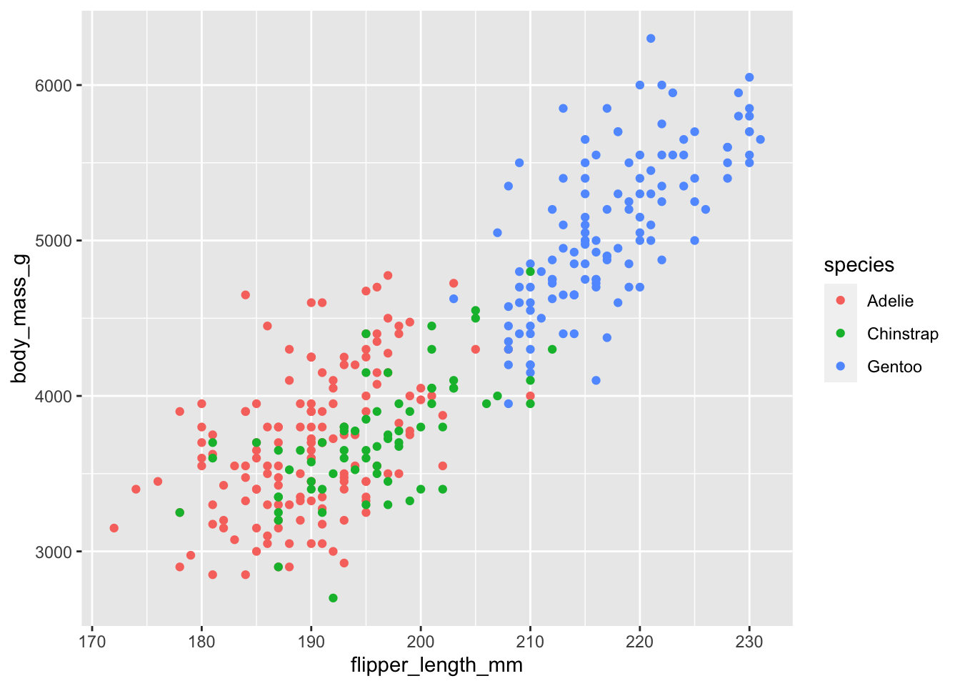
tidymodelsによるランダムフォレストのモデル構築と実行
データ分割
データを、訓練用データと検証用データとに分割します。speciesにより層化しています。
penguins_split <- initial_split(penguins, prop = 0.8, strata = species)
penguins_train <- training(penguins_split)
penguins_test <- testing(penguins_split)
レシピ
モデル式と前処理を記述します。
モデルは、説明変数 bill_length_mm, bill_depth_mm, flipper_length_mm, body_mass_g, sex により species を判別するものとなっています。
前処理として、欠測値の補完をおこなっています。
penguins_recipe <- recipe(species ~ bill_length_mm + bill_depth_mm +
                            flipper_length_mm + body_mass_g + sex,
                          data = penguins_train) %>%
  step_impute_mean(bill_length_mm, bill_depth_mm,
                   flipper_length_mm, body_mass_g) %>%
  step_impute_knn(sex)
penguins_recipe <- prep(penguins_recipe)
モデル
モデルの定義です。ランダムフォレストによる分類で、エンジンにはrangerを使用します。set_engine関数にimportance = "permutation"と引数を与えて、説明変数の重要度を計算させるようにしています。
rf_model <- rand_forest() %>%
  set_mode("classification") %>%
  set_engine("ranger", seed = 123, importance = "permutation")
ワークフロー
ワークフローを定義します。
penguins_wf <- workflow() %>%
  add_recipe(penguins_recipe) %>%
  add_model(rf_model)
あてはめ
訓練用データにモデルのあてはめを実行します。
penguins_fit <- penguins_wf %>%
  fit(data = penguins_train)
結果
結果の概要を表示します。
penguins_fit %>%
  extract_fit_parsnip()
## parsnip model object
##
## Ranger result
##
## Call:
##  ranger::ranger(x = maybe_data_frame(x), y = y, seed = ~123, importance = ~"permutation",      num.threads = 1, verbose = FALSE, probability = TRUE)
##
## Type:                             Probability estimation
## Number of trees:                  500
## Sample size:                      274
## Number of independent variables:  5
## Mtry:                             2
## Target node size:                 10
## Variable importance mode:         permutation
## Splitrule:                        gini
## OOB prediction error (Brier s.):  0.03085326
予測
検証用データを対象に予測をおこないます。
penguins_predict <- augment(penguins_fit, new_data = penguins_test)精度
精度を表示します。
penguins_predict %>%
  accuracy(truth = species, estimate = .pred_class)
## # A tibble: 1 × 3
##   .metric  .estimator .estimate
##   <chr>    <chr>          <dbl>
## 1 accuracy multiclass         1
今回の場合は、精度が1となりました。
混同行列
混同行列を表示します。
penguins_predict %>%
  conf_mat(truth = species, estimate = .pred_class)
##            Truth
## Prediction  Adelie Chinstrap Gentoo
##   Adelie        31         0      0
##   Chinstrap      0        14      0
##   Gentoo         0         0     25
今回の場合は、完全に正解となりました。
tidymodelsによるハイパーパラメータチューニング
準備
訓練用データを、交差検証用に10分割します。
penguins_cv_splits <- vfold_cv(penguins_train,
                               strata = "species",
v = 10)ハイパーパラメータチューニング用のワークフローを定義します。mtryとtreesを対象に、チューニングをおこなうようにします。
penguins_rf_cv <- workflow() %>%
  add_recipe(penguins_recipe) %>%
  add_model(rand_forest(mtry = tune(),
                        trees = tune()) %>%
              set_mode("classification") %>%
              set_engine("ranger", seed = 123,
importance = "permutation"))parametersオブジェクトを作成します。
rf_params <- list(trees(), mtry() %>%
                    finalize(penguins_recipe %>%
                               prep() %>%
                               bake(new_data = NULL) %>%
                               select(bill_length_mm, bill_depth_mm,
                                      flipper_length_mm, body_mass_g,
                                      sex))) %>%
  parameters()
print(rf_params)
## Collection of 2 parameters for tuning
##
##  identifier  type    object
##       trees trees nparam[+]
##        mtry  mtry nparam[+]
探索範囲を作成します。ランダムサーチで、探索格子点の数を50としています。
rf_grid_range <- rf_params %>%
  grid_random(size = 50)
実行
ランダムサーチを実行します。
penguins_rf_grid <- penguins_rf_cv %>%
  tune_grid(resamples = penguins_cv_splits,
            grid = rf_grid_range,
            control = control_grid(save_pred = TRUE),
            metrics = metric_set(accuracy))
結果
autoplot関数で結果を図示します。
autoplot(penguins_rf_grid)
結果の良かったハイパーパラメータの組み合わせの上位を表示します。
penguins_rf_grid_best <- penguins_rf_grid %>%
  show_best()
print(penguins_rf_grid_best)
## # A tibble: 5 × 8
##    mtry trees .metric  .estimator  mean     n std_err .config
##   <int> <int> <chr>    <chr>      <dbl> <int>   <dbl> <chr>
## 1     1  1956 accuracy multiclass 0.985    10 0.00811 Preprocessor1_Model05
## 2     1   919 accuracy multiclass 0.985    10 0.00811 Preprocessor1_Model06
## 3     1  1308 accuracy multiclass 0.985    10 0.00811 Preprocessor1_Model10
## 4     1  1538 accuracy multiclass 0.985    10 0.00811 Preprocessor1_Model16
## 5     1   946 accuracy multiclass 0.985    10 0.00811 Preprocessor1_Model20
更新
もっとも良かったハイパーパラメータの組み合わせを使ってモデルを更新します。
penguins_rf_model_best <-
  rand_forest(trees = penguins_rf_grid_best$trees[1],
              mtry =  penguins_rf_grid_best$mtry[1]) %>%
              set_mode("classification") %>%
              set_engine("ranger", seed = 123,
                         importance = "permutation")

penguins_rf_cv_last <- penguins_rf_cv %>%
  update_model(penguins_rf_model_best)

penguins_rf_last_fit <- penguins_rf_cv_last %>%
  last_fit(penguins_split)
精度を表示します。
last_accuracy <- penguins_rf_last_fit %>%
  collect_metrics()
print(last_accuracy)
## # A tibble: 2 × 4
##   .metric  .estimator .estimate .config
##   <chr>    <chr>          <dbl> <chr>
## 1 accuracy multiclass         1 Preprocessor1_Model1
## 2 roc_auc  hand_till          1 Preprocessor1_Model1
説明変数(特徴量)の重要度を表示します。
penguins_rf_last_fit %>%
  extract_fit_engine() %>%
  ranger::importance()
##    bill_length_mm     bill_depth_mm flipper_length_mm       body_mass_g
##        0.21661401        0.12748694        0.15254562        0.10546389
##               sex
##        0.03680983
図示
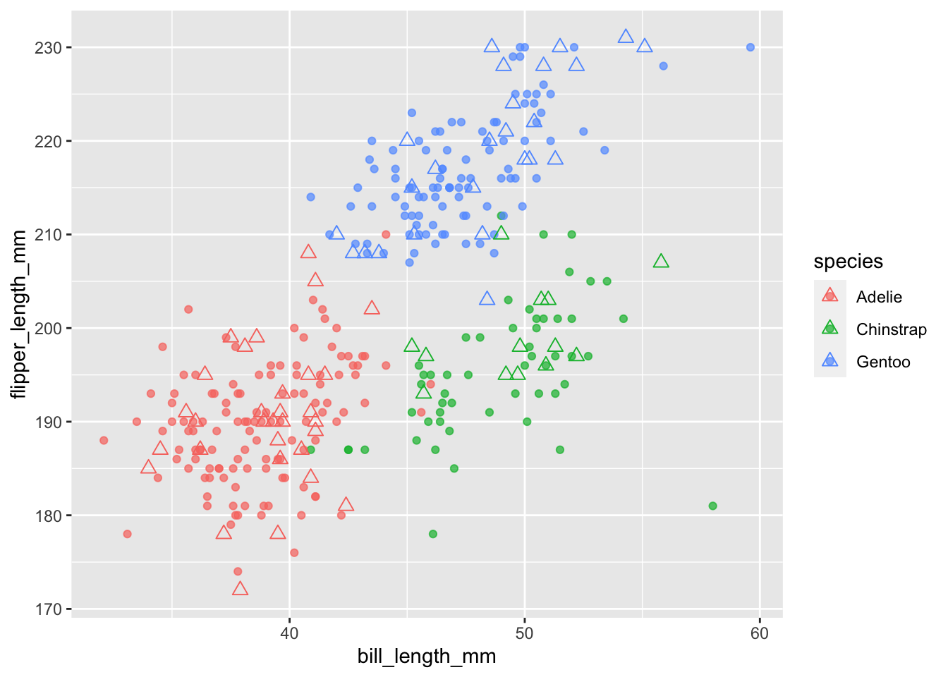
訓練用データを●で、予測した値を△で表示しました。
penguins_train %>%
  dplyr::filter(!is.na(bill_length_mm) & !is.na(flipper_length_mm)) %>%
  ggplot() +
  geom_point(aes(x = bill_length_mm, y = flipper_length_mm,
                 color = species), alpha = 0.7, size = 1.5) +
  geom_point(data = penguins_predict,
             aes(x = bill_length_mm, y = flipper_length_mm,
                 color = .pred_class), shape = 2, size = 2.5)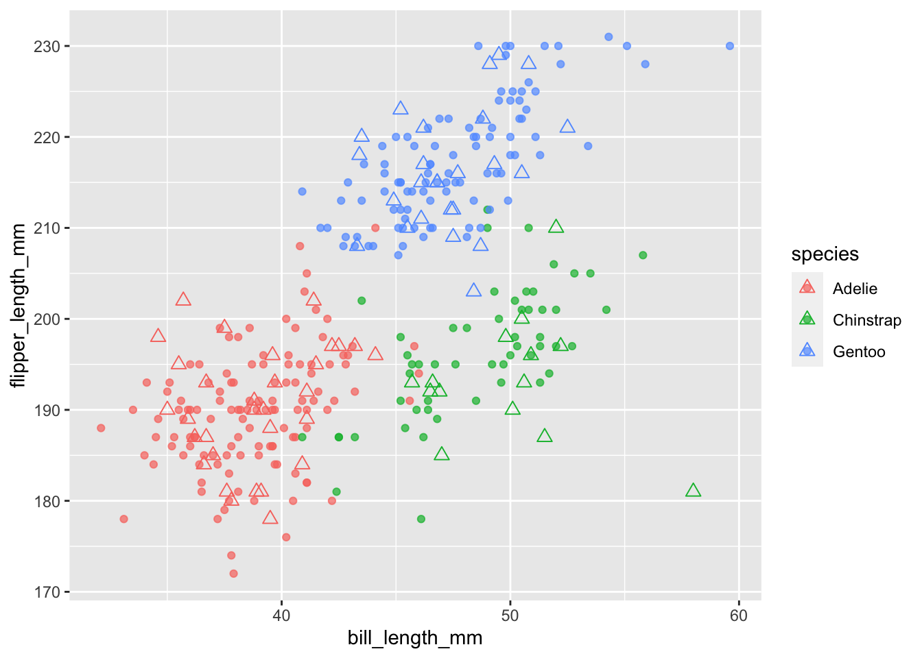
Python(reticulate経由)によるランダムフォレスト
ついでに、reticulateパッケージを使ってRStudio上でPythonを使い、同様のことをやってみました。使用するPythonは、reticulate::use_python関数や、RStudioの設定などで指定します。
Pythonのコードは、『ゼロからはじめるデータサイエンス入門 R・Python一挙両得』を参考にしています。
library(reticulate)こちらは手抜きをして、欠測値のある行を抜いています。
penguins_narm <- penguins %>%
  dplyr::select(species, bill_length_mm, bill_depth_mm,
                flipper_length_mm, body_mass_g, sex) %>%
  dplyr::filter(!is.na(bill_length_mm) &
                  !is.na(bill_depth_mm))
ランダムフォレスト
sklearnのRandomForestClassifierで、ランダムフォレストを実行します。データはRのオブジェクトを参照しています(rオブジェクトで参照できます)。
Pythonにはscikit-learnのほかpandasなどをインストールしておきます。
from sklearn.ensemble import RandomForestClassifier
from sklearn.model_selection import train_test_split

penguins_train, penguins_test = train_test_split(r.penguins_narm, test_size = 0.2,
                                                 stratify = r.penguins_narm.species)

X, y = penguins_train.iloc[:, 1:5], penguins_train.species

rf = RandomForestClassifier()
fit = rf.fit(X, y)
penguins_pred = fit.predict(penguins_test.iloc[:, 1:5])
結果
精度をみてみます。
from sklearn.metrics import accuracy_score, confusion_matrix

accuracy_score(penguins_test.species, penguins_pred)
## 0.9420289855072463
同様に混同行列です。
confusion_matrix(penguins_test.species, penguins_pred)
## array([[29,  1,  0],
##        [ 2, 12,  0],
##        [ 0,  1, 24]])
説明変数(特徴量)の重要度です。
print(fit.feature_importances_)
## [0.40918805 0.19409438 0.30000964 0.09670793]
ハイパーパラメータチューニング
LOOCVを指標としてグリッドサーチしてみます。対象のハイパーパラメータはmax_features(rangerではmtry)のみにしました。
from sklearn.model_selection import GridSearchCV, LeaveOneOut

grid = GridSearchCV(RandomForestClassifier(),
                    param_grid = {'max_features': [1, 2, 3, 4]},
                    cv = LeaveOneOut())
fit = grid.fit(X, y)
penguins_pred = fit.predict(penguins_test.iloc[:, 1:5])

print(fit.best_params_)
## {'max_features': 1}
max_features = 1が最良となりました。
それぞれのハイパーパラメータのテストスコアです。
print(fit.cv_results_['mean_test_score'])
## [0.98534799 0.98168498 0.98168498 0.97802198]
説明変数(特徴量)の重要度です。
print(fit.best_estimator_.feature_importances_)
## [0.3523138  0.19767847 0.26264029 0.18736744]
図示
PythonのオブジェクトをRから参照して、Rのときと同様に、訓練用データを●で、予測した値を△で表示しました。PythonのオブジェクトはRからはpyで参照できます。
penguins_train <- py$penguins_train
penguins_test <- py$penguins_test
penguins_test$pred <- py$penguins_pred

penguins_train |>
  dplyr::filter(!is.na(bill_length_mm) & !is.na(flipper_length_mm)) |>
  ggplot() +
  geom_point(aes(x = bill_length_mm, y = flipper_length_mm,
                 color = species), alpha = 0.7, size = 1.5) +
  geom_point(data = penguins_test,
             aes(x = bill_length_mm, y = flipper_length_mm,
                 color = pred), shape = 2, size = 2.5)