library(cmdstanr)
## This is cmdstanr version 0.7.1
## - CmdStanR documentation and vignettes: mc-stan.org/cmdstanr
## - CmdStan path: /usr/local/cmdstan
## - CmdStan version: 2.34.1
knitr::knit_engines$set(stan = cmdstanr::eng_cmdstan)
library(ggplot2)
library(posterior)
## This is posterior version 1.4.1
##
##  次のパッケージを付け加えます: 'posterior'
##  以下のオブジェクトは 'package:stats' からマスクされています:
##
##     mad, sd, var
##  以下のオブジェクトは 'package:base' からマスクされています:
##
##     %in%, match

set.seed(1234)

N <- 30
lambda <- c(1, 6, 12)
Y <- rpois(N * 3, rep(lambda, each = N))先日NIMBLEで解析した、平均が異なるポアソン分布が混合しているディリクレ過程混合モデルを今回はStanでやってみます。
データ
先日と同じく、平均が1, 6, 12のポアソン分布にしたがう計測値が混ざっている個体数データを想定して、データを生成します。
以下のようなデータになります。
ggplot(data.frame(Y = Y)) +
  geom_bar(aes(x = Y))
Stanモデル
Stanのモデルです。modelというオブジェクトに格納しておきます。
transformed parametersブロックで、折れ棒過程によりパラメータpiを計算しています。
data {
  int<lower=0> N;  // Number of sites
  int<lower=1> M;  // Maximum number of clusters
  array[N] int<lower=0> Y;  // Number of individuals
  int<lower=0> Y_max;       // maximum Y
}

parameters {
  real<lower=0> alpha;
  vector[M] phi;
  vector<lower=0, upper=1>[M - 1] q;
}

transformed parameters {
  simplex[M] pi;

  {
    real sum = 0;
    pi[1] = q[1];
    sum = pi[1];
    for (m in 2:(M - 1)) {
      pi[m] = (1 - sum) * q[m];
      sum += pi[m];
    }
    pi[M] = 1 - sum;
  }
}

model {
  for (n in 1:N) {
    vector[M] lp;
    for (m in 1:M) {
      lp[m] = bernoulli_lpmf(1 | pi[m])
              + poisson_log_lpmf(Y[n] | phi[m]);
    }
    target += log_sum_exp(lp);
  }
  phi ~ normal(0, 5);
  q ~ beta(1, alpha);
  alpha ~ gamma(1, 1);
}

generated quantities {
  vector[Y_max + 1] dens;
  matrix[Y_max + 1, M] dens_c;

  for (y in 0:Y_max) {
    for (m in 1:M) {
      real lambda = exp(phi[m]);
      dens_c[y + 1, m] = pi[m] * lambda^y * exp(-lambda) / tgamma(y + 1);
    }
    dens[y + 1] = sum(dens_c[y + 1, ]);
  }
}
あてはめ
データにモデルをあてはめます。
stan_data <- list(N = N * 3, M = 20, Y = Y, Y_max = max(Y))
fit <- model$sample(stan_data, seed = 1,
                    chains = 4, parallel_chains = 4,
                    iter_warmup = 4000, iter_sampling = 4000,
                    refresh = 0)
## Running MCMC with 4 parallel chains...
##
## Chain 3 finished in 106.7 seconds.
## Chain 2 finished in 107.2 seconds.
## Chain 1 finished in 113.2 seconds.
## Chain 4 finished in 141.6 seconds.
##
## All 4 chains finished successfully.
## Mean chain execution time: 117.2 seconds.
## Total execution time: 141.8 seconds.
結果
まずは、ベータ分布(beta(1, alpha))のパラメータのalphaです。各クラスタにはいるデータの数は同じなので、理想的には1になるはずですが、やや大きな値となりました。この値は事前分布にもかなり影響を受けるみたいです。
fit$summary("alpha")
## # A tibble: 1 × 10
##   variable  mean median    sd   mad    q5   q95  rhat ess_bulk ess_tail
##   <chr>    <num>  <num> <num> <num> <num> <num> <num>    <num>    <num>
## 1 alpha     1.35   1.19 0.709 0.602 0.538  2.72  1.00    2511.    4388.
各クラスタが選ばれる確率です。データでは3クラスタですが、結果でも3クラスタ目までの確率が比較的たかくなっています。
pi_est <- fit$summary("pi") |>
  dplyr::mutate(index = stringr::str_extract(variable, "[0-9]+") |>
                  as.numeric() |> as.factor())
ggplot(pi_est) +
  geom_point(aes(x = index, y = mean)) +
  geom_segment(aes(x = index, xend = index, y = q5, yend = q95)) +
  labs(x = "Component", y = "Probability")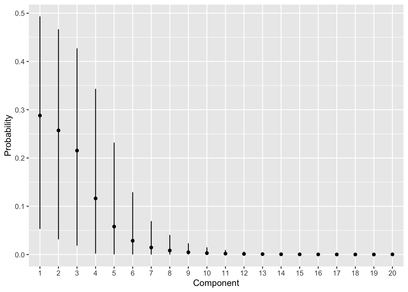
各個体数の密度分布をデータと推定値とで比較します。だいたいのところは再現できているようです。
dens <- fit$summary("dens") |>
  dplyr::mutate(Y = stringr::str_extract(variable, "[0-9]+") |>
                  as.numeric() - 1)
ggplot(dens) +
  geom_bar(data = data.frame(Y = Y), aes(x = Y, y = after_stat(prop))) +
  geom_point(aes(x = Y, y = mean), colour = "red", size = 1.5) +
  geom_segment(aes(x = Y, xend = Y, y = q5, yend = q95),
              colour = "red")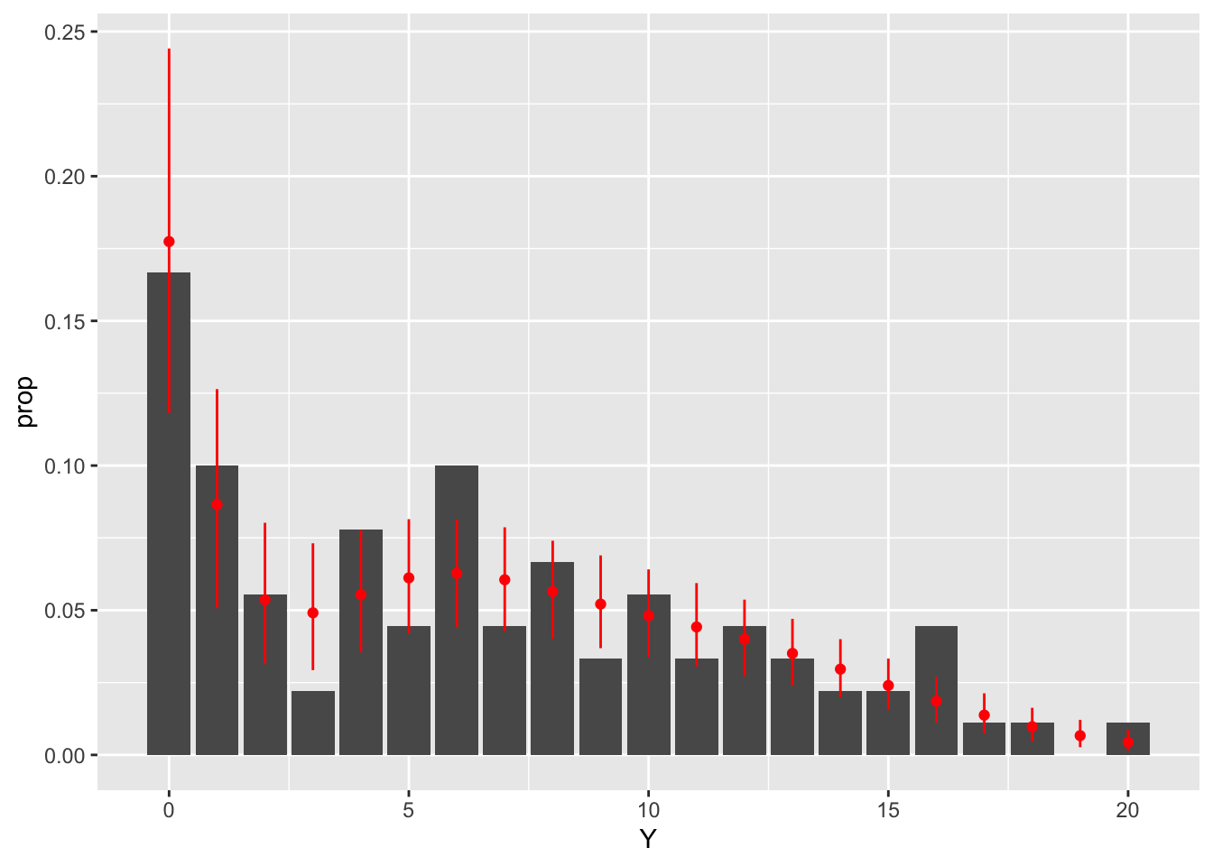
参考
StatModeling Memorandum ノンパラベイズ(ディリクレ過程)の実装
The Stan Forums Better way of modeling stick-breaking process