library(rjags)
## 要求されたパッケージ coda をロード中です
## Linked to JAGS 4.3.2
## Loaded modules: basemod,bugs
library(readr)
library(dplyr)
##
## 次のパッケージを付け加えます: 'dplyr'
## 以下のオブジェクトは 'package:stats' からマスクされています:
##
##     filter, lag
## 以下のオブジェクトは 'package:base' からマスクされています:
##
##     intersect, setdiff, setequal, union
library(tidyr)
library(stringr)
library(ggplot2)
library(posterior)
## This is posterior version 1.5.0
##
## 次のパッケージを付け加えます: 'posterior'
## 以下のオブジェクトは 'package:stats' からマスクされています:
##
##     mad, sd, var
## 以下のオブジェクトは 'package:base' からマスクされています:
##
##     %in%, match
library(bayesplot)
## This is bayesplot version 1.11.1
## - Online documentation and vignettes at mc-stan.org/bayesplot
## - bayesplot theme set to bayesplot::theme_default()
##    * Does _not_ affect other ggplot2 plots
##    * See ?bayesplot_theme_set for details on theme setting
##
## 次のパッケージを付け加えます: 'bayesplot'
## 以下のオブジェクトは 'package:posterior' からマスクされています:
##
##     rhat

set.seed(123)松浦健太郎さんの“Bayesian Statistical Modeling with Stan, R, and Python”の11.5節にある、変化点(スイッチ成分)を持つ状態空間モデルをJAGSに移植してみました。
準備
ライブラリの読み込みと乱数の設定です。
データ
データを読み込んで整形します。ここは、CSVファイルをGitHubから読み込むところ以外は、サンプルコードとほぼ同じです。
data_url <- "https://raw.githubusercontent.com/MatsuuraKentaro/Bayesian_Statistical_Modeling_with_Stan_R_and_Python/master/chap11/input/data-eg1.csv"
d <- read_csv(data_url) |>
  tidyr::pivot_wider(id_cols = c(Group, PID),
                     names_from = Time,
                     values_from = Y)
## Rows: 1680 Columns: 4
## ── Column specification ────────────────────────────────────────────────────────
## Delimiter: ","
## dbl (4): Group, PID, Time, Y
##
## ℹ Use `spec()` to retrieve the full column specification for this data.
## ℹ Specify the column types or set `show_col_types = FALSE` to quiet this message.
Y1 <- d |>
  dplyr::filter(Group == 1) |>
  dplyr::select(-Group, -PID)
Y2 <- d |>
  dplyr::filter(Group == 2) |>
  dplyr::select(-Group, -PID)
T <- ncol(Y1)
N1 <- nrow(Y1)
N2 <- nrow(Y2)
data <- list(T = T, N1 = N1, N2 = N2, Y1 = Y1, Y2 = Y2)
モデル
JAGSのモデルです。元のStanのコードをほとんどそのままJAGSに移植していますが、スケールパラメータの事前分布は、収束を良くするため弱情報事前分布にしてあります。
分布の引数に式を使っているので、Win/OpenBUGSでは動作しません。NIMBLEでは動作するでしょう。
model_file <- "model11-10.txt"
readLines(model_file) |>
  cat(sep = "\n")
## #
## # model11-10.txt
## #
##
## model {
##   # observation model
##   for (n in 1:N1) {
##     for (t in 1:T) {
##       Y1[n, t] ~ dnorm(trend[t], tau_y)
##     }
##   }
##   for (n in 1:N2) {
##     for (t in 1:T) {
##       Y2[n, t] ~ dnorm(trend[t] + sw[t], tau_y)
##     }
##   }
##
##   # system model
##   # trend component
##   for (t in 1:2) {
##     trend[t] ~ dnorm(0, 1)
##   }
##   for (t in 3:T) {
##     trend[t] ~ dnorm(2 * trend[t - 1] - trend[t - 2], tau_trend)
##   }
##
##   # switch component
##   sw[1] <- sw_ini;
##   for (t in 2:T) {
##     sw[t] <- sw[t - 1] + s_sw * tan(sw_unif[t - 1])
##   }
##   for (t in 1:(T - 1)) {
##     sw_unif[t] ~ dunif(-3.141592 / 2, 3.141592 / 2)
##   }
##   sw_ini ~ dnorm(0, 1)
##
##   # scale parameters
##   tau_y <- 1 / (s_y * s_y)
##   s_y ~ dnorm(0, 1) T(0, )
##   tau_trend <- 1 / (s_trend * s_trend)
##   s_trend ~ dnorm(0, 1) T(0, )
##   s_sw ~ dnorm(0, 1) T(0, )
## }
JAGS実行
実行します。モデルのアダプテーションに1000回、その後2000回のバーンインを設けています。サンプリングは、10000回繰り返し中10ごとに間引いておこなっています。詳細はあとでも出てきますが、スイッチ成分のスケールs_swの収束が、Stanにくらべると良くないです。
model <- jags.model(model_file, data = data,
                    n.chains = 3, n.adapt = 1000)
## Compiling model graph
##    Resolving undeclared variables
##    Allocating nodes
## Graph information:
##    Observed stochastic nodes: 1680
##    Unobserved stochastic nodes: 51
##    Total graph size: 1882
##
## Initializing model
update(model, 2000)
fit <- coda.samples(model,
                    variable = c("trend", "sw",
                                 "s_y", "s_trend", "s_sw"),
                    n.iter = 10000, thin = 10) |>
  as_draws()
結果
R-hatを確認します。大きい順に並べ替えて表示します。
fit |>
  summarise_draws() |>
  dplyr::arrange(desc(rhat)) |>
  dplyr::select(variable, rhat)
## # A tibble: 51 × 2
##    variable   rhat
##    <chr>     <dbl>
##  1 s_sw       1.05
##  2 sw[6]      1.01
##  3 sw[5]      1.01
##  4 sw[7]      1.01
##  5 sw[17]     1.00
##  6 sw[18]     1.00
##  7 sw[13]     1.00
##  8 trend[11]  1.00
##  9 sw[22]     1.00
## 10 sw[16]     1.00
## # ℹ 41 more rows
いちおうすべてのパラメータで1.1未満となっていました。
R-hat値が最も大きかったs_swの軌跡を確認してみます。
mcmc_trace(fit, pars = "s_sw")
各連鎖はとりあえず混ざっていますが、まだちょっと自己相関が残っているようでした。
グラフ表示
状態パラメータのトレンド成分trendとスイッチ成分swの推定結果を表示します。
まず、各パラメータについて各時点の分位点の値を取り出します。
q <- fit |>
  summarise_draws(~quantile(.x, probs = c(0.025, 0.25, 0.5,
                                          0.75, 0.975)))
trend <- q |>
  dplyr::filter(str_detect(variable, "^trend\\[[0-9]+\\]")) |>
  dplyr::bind_cols(data.frame(Time = 0:(T - 1)))
sw <- q |>
  dplyr::filter(str_detect(variable, "^sw\\[[0-9]+\\]")) |>
dplyr::bind_cols(data.frame(Time = 0:(T - 1)))trend成分をプロットします。
ggplot(trend, aes(x = Time)) +
  geom_ribbon(aes(ymin = `2.5%`, ymax = `97.5%`),
              fill = "gray80") +
  geom_ribbon(aes(ymin = `25%`, ymax = `75%`),
              fill = "gray60") +
  geom_line(aes(y = `50%`)) +
  geom_point(aes(y = `50%`)) +
  labs(x = "Time", y = "Y") +
  theme_bw()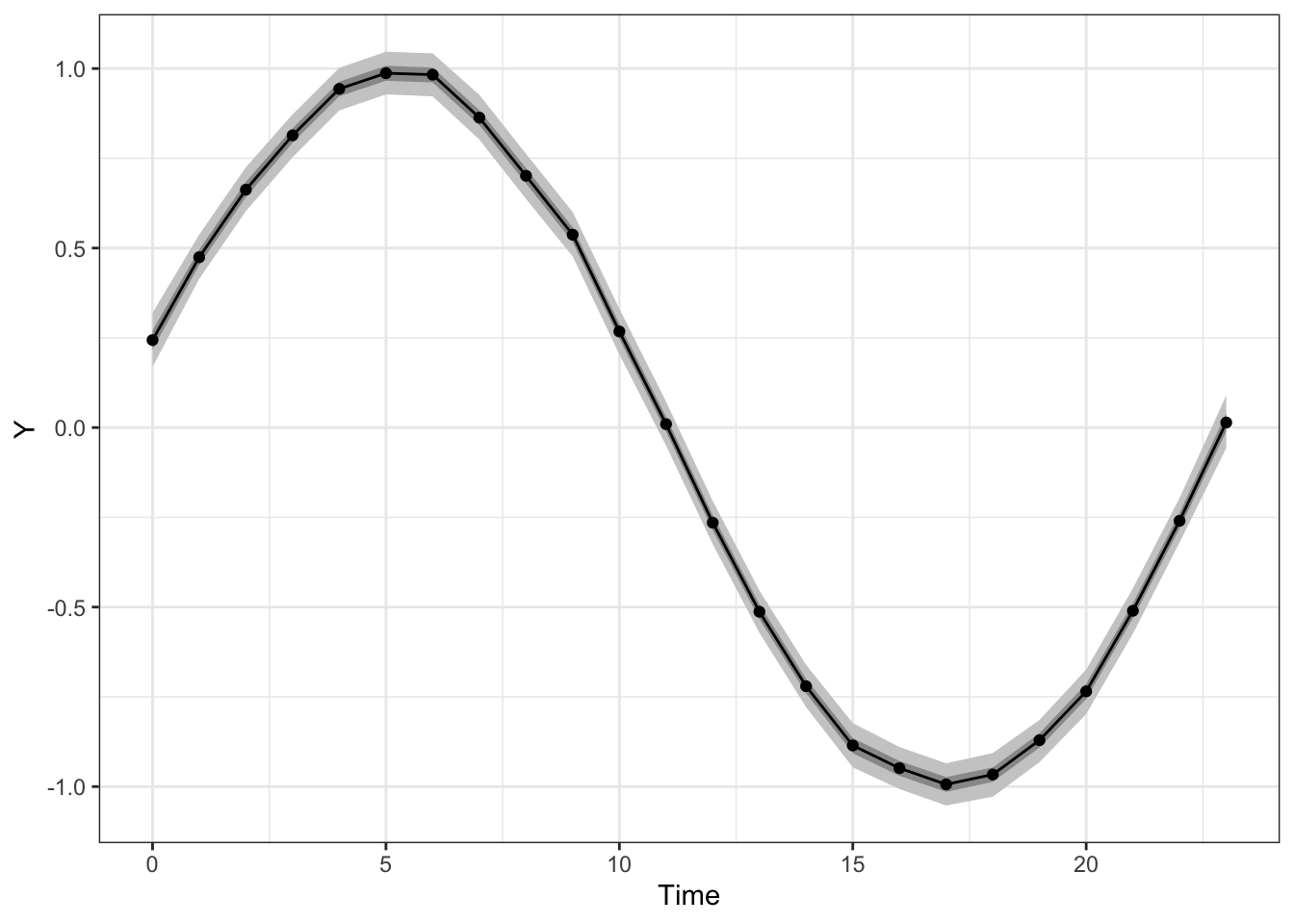
続いて、swをプロットします。
ggplot(sw, aes(x = Time)) +
  geom_ribbon(aes(ymin = `2.5%`, ymax = `97.5%`),
              fill = "gray80") +
  geom_ribbon(aes(ymin = `25%`, ymax = `75%`),
              fill = "gray60") +
  geom_line(aes(y = `50%`)) +
  geom_point(aes(y = `50%`)) +
  labs(x = "Time", y = "Y") +
  theme_bw()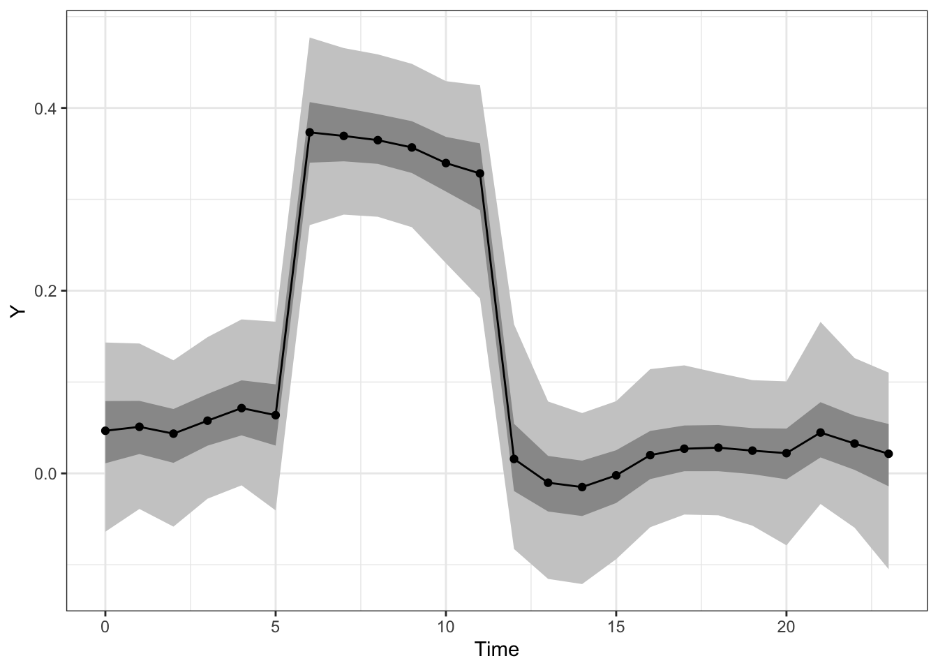
s_swの収束は、Stanと比べて良くなかったのですが、両パラメータの推定値はほぼStanによる結果と同様でした。