library(sf)
## Linking to GEOS 3.11.0, GDAL 3.5.3, PROJ 9.1.0; sf_use_s2() is TRUE
library(spdep)
## 要求されたパッケージ spData をロード中です
## To access larger datasets in this package, install the spDataLarge
## package with: `install.packages('spDataLarge',
## repos='https://nowosad.github.io/drat/', type='source')`
library(ggplot2)
library(readr)
library(stringr)

jp_font <- "IPAexGothic"前回の記事で用いた石川県の市町村人口データについて、空間自己相関の指標となるモランのI統計量 (Moran’s I statistic) を計算してみます。
準備
必要なパッケージを読み込みます。spdepパッケージは、隣接リストを作成するpoly2nb関数と、モランのI統計量を計算するmoran.test関数のため必要です。
データ
データは前回と同じですが、市町村ごとにジオメトリをまとめたdata2で、行を市町村コード順に並べ替えておきました。
data_file <- file.path("data", "N03-20240101_17.geojson")
data <- st_read(data_file)
## Reading layer `N03-20240101_17' from data source
##   `/Users/hiroki/Sites/www/posts/2024-08-22-Morans-I/data/N03-20240101_17.geojson'
##   using driver `GeoJSON'
## Simple feature collection with 1710 features and 6 fields
## Geometry type: POLYGON
## Dimension:     XY
## Bounding box:  xmin: 136.242 ymin: 36.06723 xmax: 137.3653 ymax: 37.85791
## Geodetic CRS:  WGS 84
name_code <- as.data.frame(data) |>
  dplyr::select(N03_004, N03_007) |>
  dplyr::distinct()
data2 <- data |>
  dplyr::group_by(N03_004) |>
  dplyr::summarise(geometry = st_union(geometry)) |>
  dplyr::ungroup() |>
  dplyr::left_join(name_code, by = "N03_004") |>
  dplyr::arrange(N03_007) |>
  dplyr::rename(name = N03_004,
                code = N03_007)
人口データ
こちらも前回と同様に人口データを準備します。
pop_data_file <- file.path("data", "FEI_CITY_240820142223.csv")
pop_data <- read_csv(pop_data_file, skip = 4,
                     col_types = "cc_n",
                     col_names = c("year", "name", "population")) |>
  dplyr::mutate(name = str_sub(name, str_locate(name, " ")[1] + 1)) |>
  dplyr::filter(year == "2020年度")
プロット
図示して確認します。
data2 |>
  dplyr::left_join(pop_data, by = "name") |>
ggplot() +
  geom_sf(aes(fill = population)) +
  geom_sf_text(aes(label = name), size = 2.5, family = jp_font) +
  scale_x_continuous(breaks = seq(136.5, 137.5, 0.5)) +
  scale_fill_gradient(name = "人口",
                      low = "skyblue",
                      high = "red",
                      transform = "log",
                      limits = c(5e+3, 5e+5),
                      breaks = c(5e+3, 1e+4, 5e+4, 1e+5, 5e+5),
                      labels = c("5000", "1万", "5万",
                                 "10万", "50万")) +
  labs(x = NULL, y = NULL) +
  theme_bw(base_family = jp_font)
隣接リストの作成
poly2nb関数で隣接リストを作成します。queen引数を省略しているので、デフォルト値でqueen=TRUEとなり、点で接するポリゴンも隣接関係にあるとされますが、今回のデータではTRUEでもFALSEでも変わりありません。
nb <- poly2nb(data2)プロット
地図で隣接関係を確認します。
coordには、各ポリゴンの重心の座標を入れています。3〜5行目では、隣接リストnbを、nb2lines関数で隣接するポリゴン間を結ぶベクトルデータにして、それをas関数でsf形式に変換し、CRSにWGS84を指定したものをlinesオブジェクトに代入するということをしています。
coord <- st_centroid(data2) |>
  st_coordinates()
lines <- nb |>
  nb2lines(coords = coord) |>
  as("sf") |>
  st_set_crs("WGS84")
ggplot() +
  geom_sf(data = data2) +
  geom_sf(data = lines, color = "blue") +
  theme_void()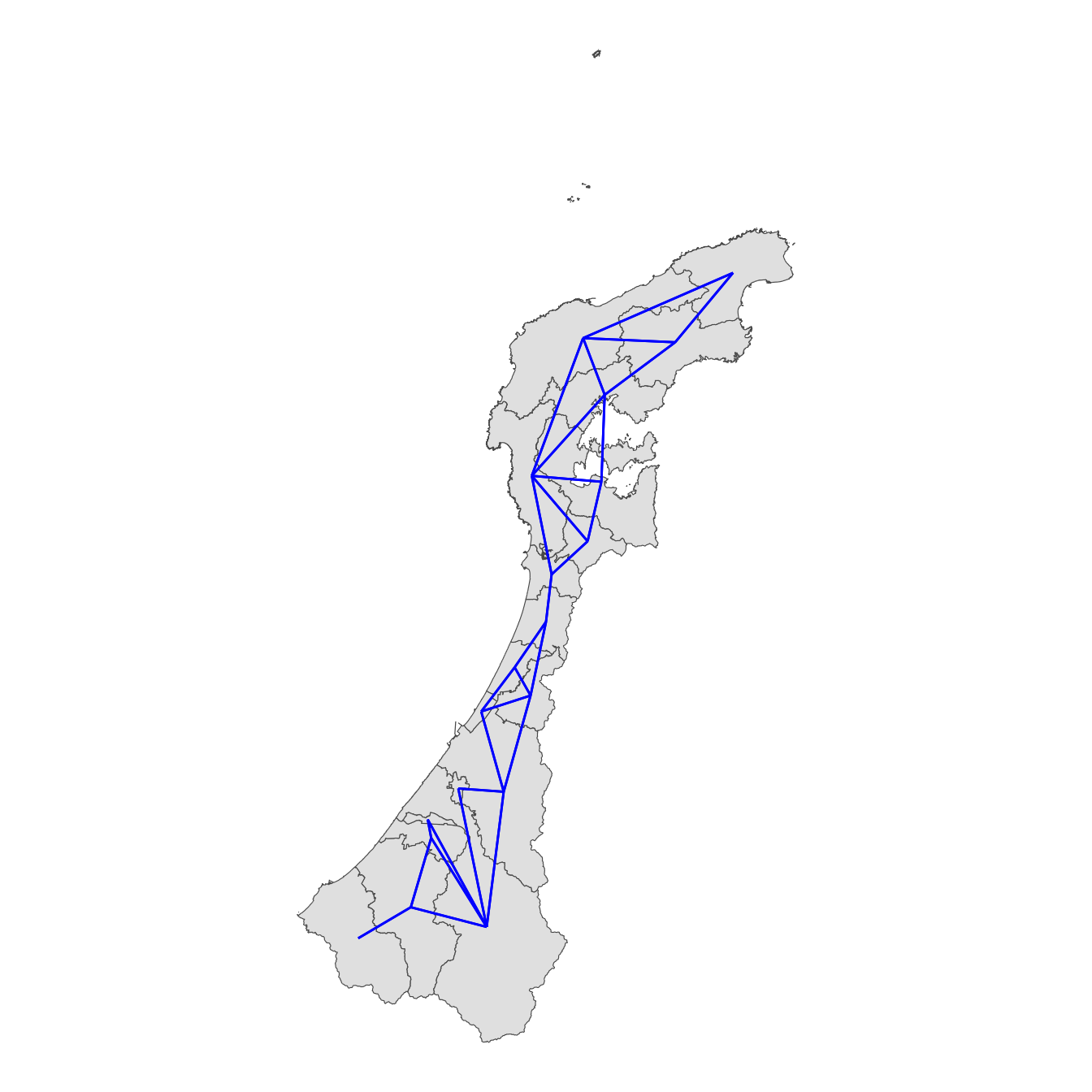
モランのI統計量
モランのI統計量を計算します。nb2listwはnbクラスの隣接リストをlistwクラスに変換する関数で、style = "W"とすると、隣接行列が行ごとに標準化されます。
moran.test(pop_data$population, nb2listw(nb, style = "W"))
##
##  Moran I test under randomisation
##
## data:  pop_data$population
## weights: nb2listw(nb, style = "W")
##
## Moran I statistic standard deviate = 1.4432, p-value = 0.07448
## alternative hypothesis: greater
## sample estimates:
## Moran I statistic       Expectation          Variance
##       0.057372548      -0.055555556       0.006122734
モランのI統計量の値は0.057で、p値も0.074という結果でした。石川県の市町村人口分布については空間自己相関はあまり大きくないようです。