tmapパッケージによる地図化 – 伊東生態統計研究室

tmapは地理空間データを地図化するパッケージで、ggplot2のように”+“演算子でレイヤーを重ねていけるのが特長です。

今回参考にしたところ

準備

sfパッケージとtmapパッケージを読み込んでおきます。

データは、国土数値情報の行政区域データの石川県の2024年のものと、鉄道時系列データの2024年のものをダウンロードして、dataフォルダにいれておきます。

また、石川県の市町村名を市区町村コード順にベクトルにいれておきます。

library(sf)
## Linking to GEOS 3.11.0, GDAL 3.5.3, PROJ 9.1.0; sf_use_s2() is TRUE
library(tmap)
## Breaking News: tmap 3.x is retiring. Please test v4, e.g. with
## remotes::install_github('r-tmap/tmap')

pref_data_file <- "data/N03-20240101_17.geojson"
rail_data_file <- "data/N05-23_RailroadSection2.geojson"
names <- c("金沢市", "七尾市", "小松市", "輪島市", "珠洲市", "加賀市",
           "羽咋市", "かほく市", "白山市", "能美市", "野々市市", "川北町",
           "津幡町", "内灘町", "志賀町", "宝達志水町", "中能登町", "穴水町",
           "能登町")

データ読み込み

データを読み込みます。読み込んだデータは座標参照系をJGD2011平面直角座標系VIIに変換します。その後、dplyrで型や名前を変換します。

鉄道データは、sf::st_intersectionで、石川県の部分を切り出しています。

pref_data <- sf::st_read(pref_data_file) |>
  sf::st_transform(crs = 6675) |>  # JGD2011平面直角座標系VII
  dplyr::mutate(`市町村` = factor(N03_004, levels = names))
## Reading layer `N03-20240101_17' from data source 
##   `/Users/hiroki/Sites/www/posts/2025-02-15-tmap/data/N03-20240101_17.geojson' 
##   using driver `GeoJSON'
## Simple feature collection with 1710 features and 6 fields
## Geometry type: POLYGON
## Dimension:     XY
## Bounding box:  xmin: 136.242 ymin: 36.06723 xmax: 137.3653 ymax: 37.85791
## Geodetic CRS:  WGS 84
rail_data <- sf::st_read(rail_data_file) |>
  sf::st_transform(crs = 6675) |> # JGD2011平面直角座標系VII
  sf::st_intersection(pref_data) |>
  dplyr::mutate_at(dplyr::vars("N05_004", "N05_005b", "N05_005e"), as.numeric) |>
  dplyr::rename(`運営会社` = N05_003)
## Reading layer `N05-23_RailroadSection2' from data source 
##   `/Users/hiroki/Sites/www/posts/2025-02-15-tmap/data/N05-23_RailroadSection2.geojson' 
##   using driver `GeoJSON'
## Simple feature collection with 2628 features and 11 fields
## Geometry type: LINESTRING
## Dimension:     XY
## Bounding box:  xmin: 127.6523 ymin: 26.19315 xmax: 145.7539 ymax: 45.41634
## Geodetic CRS:  WGS 84
## Warning: attribute variables are assumed to be spatially constant throughout
## all geometries

地図化

tmapのモードを設定します。インタラクティブにもできますが（mode = "view"）、今回は通常のグラフィックとして描画します（デフォルト）。

tmap_mode("plot")
## tmap mode set to plotting

まずは石川県の市町村を地図化してみます。

tm_shape(pref_data) +
  tm_polygons("市町村") +
  tm_layout(legend.outside = TRUE, fontfamily = "YuGothic")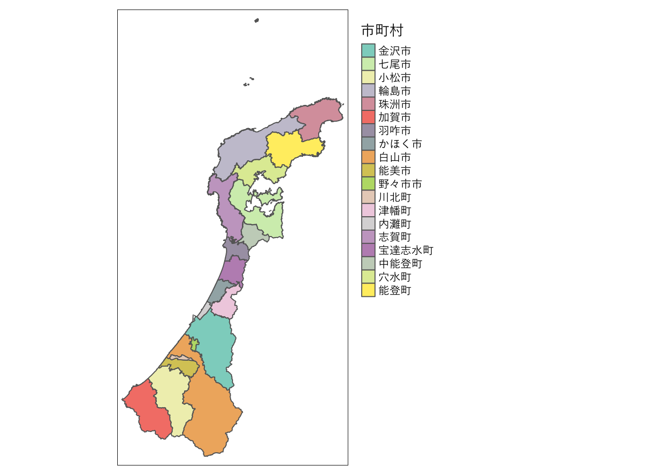

次に鉄道路線データを表示してみます。2023年現在で現存するものだけを抜き出して表示しています。

rail2023 <- rail_data |>
  dplyr::filter(N05_005e == 9999)  # 現存するもの
tm_shape(pref_data) +
  tm_polygons(col = "gray95") +
  tm_shape(rail2023) +
  tm_lines("運営会社", lwd = 2, palette = palette("Okabe_Ito")) +
  tm_layout(legend.outside = TRUE, fontfamily = "YuGothic")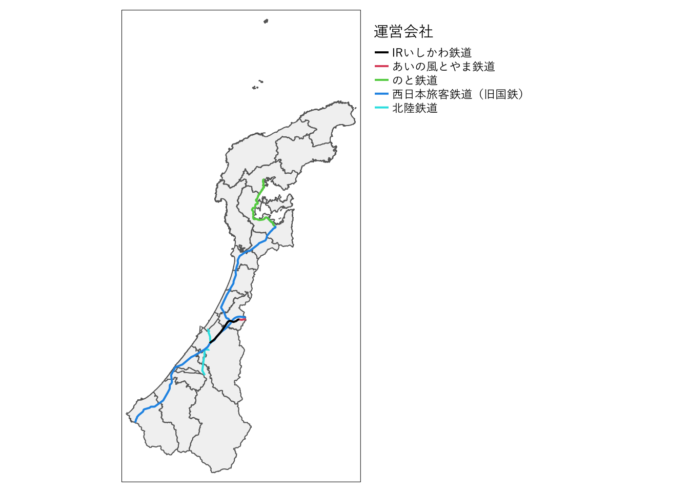

続いて、1960年に現存していたものを表示してみます。

rail1960 <- rail_data |>
  dplyr::filter(N05_005b <= 1960, N05_005e > 1960)  # 1960年
tm_shape(pref_data) +
  tm_polygons(col = "gray95") +
  tm_shape(rail1960) +
  tm_lines("運営会社", lwd = 2, palette = palette("Okabe-Ito")) +
  tm_layout(legend.outside = TRUE, fontfamily = "YuGothic")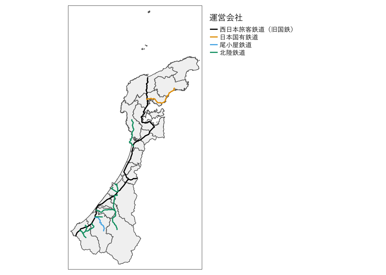

おわりに

静的な地図ならggplot2のgeom_sfでもできますので、今回の内容はあまりtmapの真価を発揮できていないかもしれません。拡大・縮小・移動できる地図に地理空間データを簡単に載せられるのがtmapの便利なところなのでしょう。