BPA第5章イワツバメのデータをつかって、KFASで状態空間モデルのあてはめ

Bayesian Population Analysis using WinBUGS 第5章のイワツバメのデータをつかって、KFASで状態空間モデルのあてはめをおこないます。KFASでは、観測値が正規分布以外の分布も扱うことができます。

なお、この本の日本語訳は以下になります。

準備

使用するパッケージを読み込み、データをデータフレームに入れます。

データは、スイス北部マグデン村で1990年から観測された繁殖つがい数です。

library(ggplot2)
library(KFAS)
## Please cite KFAS in publications by using: 
## 
##   Jouni Helske (2017). KFAS: Exponential Family State Space Models in R. Journal of Statistical Software, 78(10), 1-39. doi:10.18637/jss.v078.i10.

hm_data <- data.frame(year = 1990:2009,
                      n_pairs = c(271, 261, 309, 318, 231,
                                  216, 208, 226, 195, 226,
                                  233, 209, 226, 192, 191,
                                  225, 245, 205, 191, 174))

データ確認

データを図示して確認します。

ggplot(hm_data, aes(x = year, y = n_pairs)) +
  geom_line() +
  labs(x = "Year", y = "Number of pairs")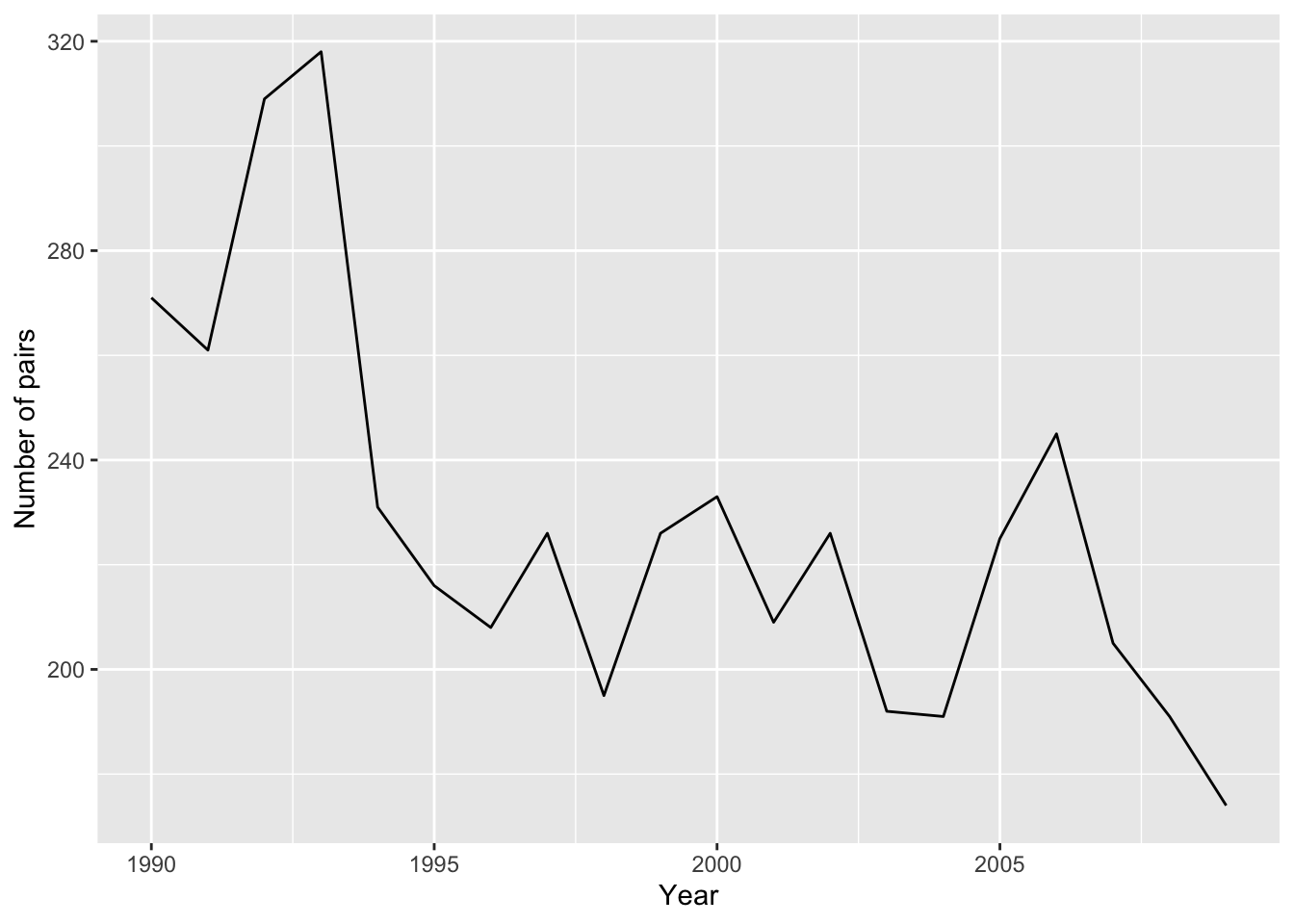

モデル

KFASでローカルトレンドモデルを定義します。状態方程式の分散を推定するようにします。

model <- SSModel(n_pairs ~ SSMtrend(degree = 2,
                                    Q = list(matrix(NA), matrix(NA))),
                 data = hm_data, distribution = "poisson")

モデルをデータにあてはめます。

fit <- fitSSM(model, inits = c(1, 1), method = "BFGS")

結果

推定された状態方程式の分散共分散行列(Q)を表示します。

fit$model$Q
## , , 1
## 
##             [,1]         [,2]
## [1,] 0.009777207 0.000000e+00
## [2,] 0.000000000 1.424109e-07

平滑化された状態の値（level成分とslope成分）を表示します。

KFS(fit$model) |>
  coef(filtered = FALSE)
## Time Series:
## Start = 1 
## End = 20 
## Frequency = 1 
##       level       slope
##  1 5.608739 -0.02219142
##  2 5.604090 -0.02219167
##  3 5.700414 -0.02219366
##  4 5.697258 -0.02219592
##  5 5.492649 -0.02219552
##  6 5.401490 -0.02219412
##  7 5.365687 -0.02219251
##  8 5.387129 -0.02219155
##  9 5.334758 -0.02219015
## 10 5.400136 -0.02219002
## 11 5.420438 -0.02219051
## 12 5.371030 -0.02219060
## 13 5.380261 -0.02219115
## 14 5.300501 -0.02219086
## 15 5.301470 -0.02219091
## 16 5.394313 -0.02219264
## 17 5.439224 -0.02219534
## 18 5.335534 -0.02219686
## 19 5.256944 -0.02219755
## 20 5.187076 -0.02219755

観測値のスケールで平滑化された値（赤線）を観測値（黒線）に重ねて図示します。

pred1 <- predict(fit$model, type = "response",
                            interval = "confidence", level = 0.95,
                            nsim = 1000)
hm_data$fit <- pred1[, "fit"]
hm_data$lwr <- pred1[, "lwr"]
hm_data$upr <- pred1[, "upr"]

p1 <- ggplot(hm_data) +
  geom_line(aes(x = year, y = n_pairs),
            color = "black", linewidth = 1) +
  geom_line(aes(x = year, y = fit), color = "red", linewidth = 1) +
  geom_ribbon(aes(x = year, ymin = lwr, ymax = upr),
              fill = "red", alpha = 0.5) +
  labs(x = "Year", y = "Number of pairs")
plot(p1)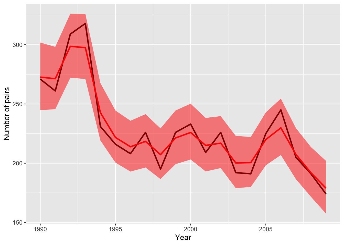

予測

6年先までの予測値を求め、95％信頼区間とともに図示します（橙色）。

last_year <- max(hm_data$year)
pred_years <- 6
pred2 <- predict(fit$model, n.ahead = pred_years,
                 interval = "confidence", level = 0.95,
                 type = "response",
                 nsim = 1000)
pred_last <- hm_data |>
               tail(1)
hm_pred <- data.frame(year = last_year:(last_year + pred_years),
                      prediction = c(pred_last[, "fit"], pred2[, "fit"]),
                      lower = c(pred_last[, "lwr"], pred2[, "lwr"]),
                      upper = c(pred_last[, "upr"], pred2[, "upr"]))

p1 +
  geom_line(data = hm_pred,
            aes(x = year, y = prediction),
            color = "red", linewidth = 1) +
  geom_ribbon(data = hm_pred,
              aes(x = year, ymin = lower, ymax = upper),
              fill = "red", alpha = 0.5)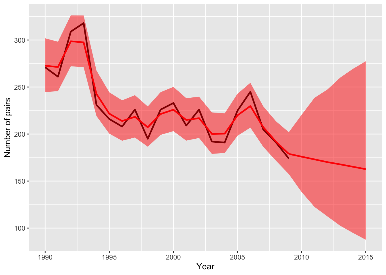

結果は元の本の、WinBUGSで推定したものとだいたい同じになりました。