library(ordinal)
library(extraDistr)
##
## 次のパッケージを付け加えます: 'extraDistr'
## 以下のオブジェクトは 'package:ordinal' からマスクされています:
##
##     dgumbel, pgumbel, qgumbel, rgumbel
library(ggplot2)

set.seed(1234)

# inverse logit function
inv_logit <- function(x) {
  1 / (1 + exp(-x))
}変量効果(random effect)のある順序ロジスティック回帰(ordered logistic regression)です。Rでは以前はdrmパッケージがあったのですが、現在はCRANから消えてしまっています。そのかわりというわけでもないですが、現在はordinalパッケージのclmm関数を使うことができます。
データ
まずはパッケージの読み込みと乱数シードの設定をおこない、逆ロジット関数を定義します。
模擬データを生成します。説明変数xは一様乱数から生成します。10個の群があり、これによる変量効果が加わるとします。ロジットスケールでの傾きをbetaに代入しておきます。
N_group <- 10
N <- N_group * 30

beta <- 1.4
x <- runif(N, -4, 4)
group <- rep(seq_len(N_group), each = N / N_group)
ranef <- rnorm(N_group, 0, 1)目的変数yは5つのカテゴリーからなる順序尺度変数とします。カテゴリー間のカットポイントの値をcpに代入しておきます。各カテゴリー以上となる確率を計算しrcat関数でカテゴリー分布の乱数でyを生成します。
cp <- c(0, 0.8, 1.7, 2)
K <- length(cp) + 1
p <- matrix(0, ncol = K, nrow = N)
p[, 1] <- 1 - inv_logit(beta * x - cp[1] + ranef[group])
for (k in 2:(K - 1)) {
  p[, k] <- inv_logit(beta * x  - cp[k - 1]+ ranef[group]) -
    inv_logit(beta * x - cp[k] + ranef[group])
}
p[, K] <- inv_logit(beta * x - cp[K - 1] + ranef[group])
y <- sapply(1:N, function(j) rcat(1, p[j, ]))
最後にデータフレームにまとめます。
data <- data.frame(x = x, y = ordered(y), group = factor(group))データをプロットして確認します。
ggplot(data, aes(x = x, y = y)) +
  geom_point(aes(colour = group))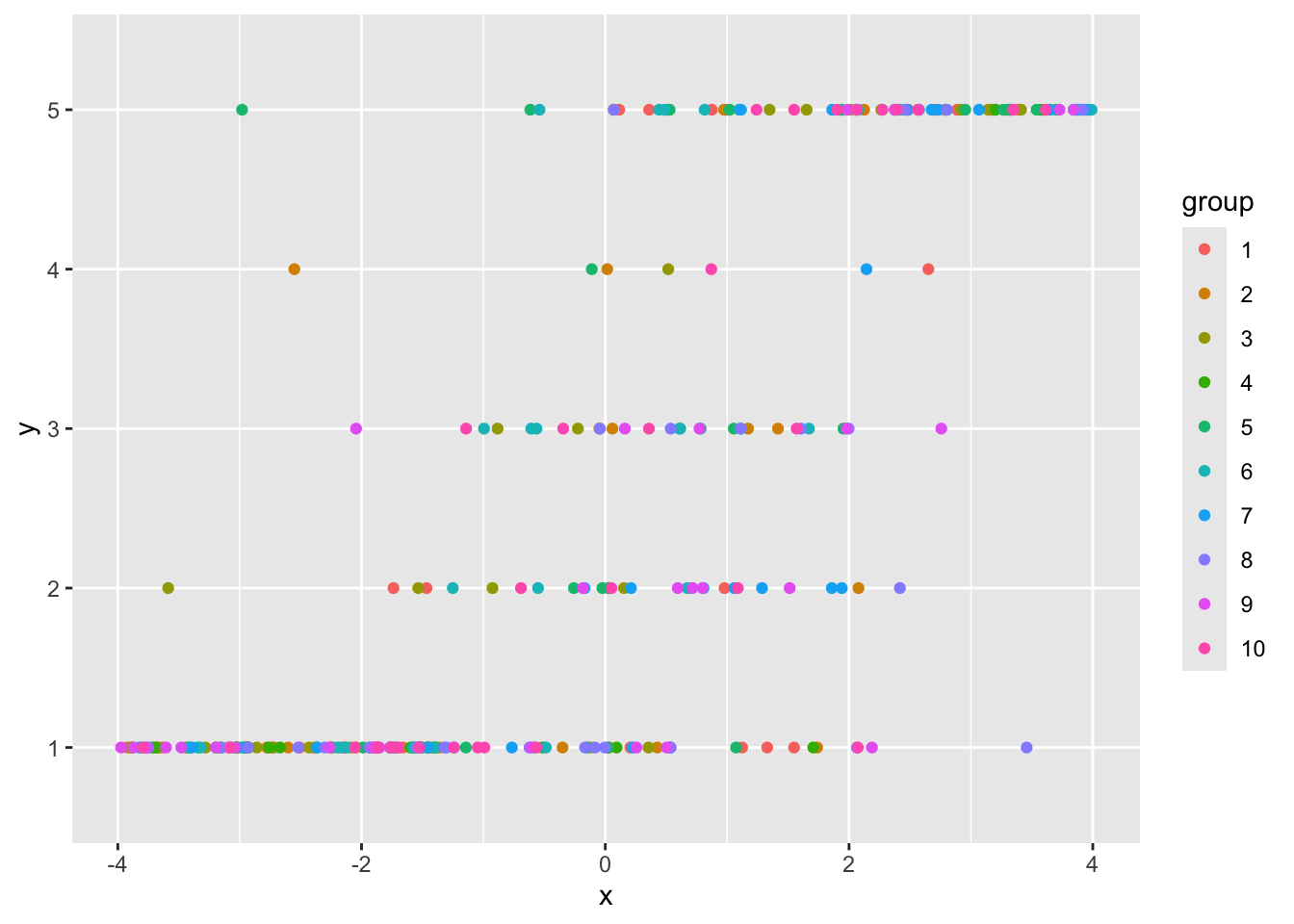
ordinal::clmmによるロジスティック回帰
clmm関数によるロジスティック回帰です。変量効果を含むモデル式の記法は、lme4::lmerなどと同様です。
fit_clmm <- clmm(y ~ x + (1|group), data = data, link = "logit")結果
結果を確認します。模擬データを生成した値と近い値が推定されました。
summary(fit_clmm)
## Cumulative Link Mixed Model fitted with the Laplace approximation
##
## formula: y ~ x + (1 | group)
## data:    data
##
##  link  threshold nobs logLik  AIC    niter    max.grad cond.H
##  logit flexible  300  -242.25 496.51 295(888) 1.39e-04 6.2e+01
##
## Random effects:
##  Groups Name        Variance Std.Dev.
##  group  (Intercept) 0.4011   0.6334
## Number of groups:  group 10
##
## Coefficients:
##   Estimate Std. Error z value Pr(>|z|)
## x    1.285      0.113   11.37   <2e-16 ***
## ---
## Signif. codes:  0 '***' 0.001 '**' 0.01 '*' 0.05 '.' 0.1 ' ' 1
##
## Threshold coefficients:
##     Estimate Std. Error z value
## 1|2  -0.2647     0.2670  -0.992
## 2|3   0.6986     0.2699   2.588
## 3|4   1.6881     0.2902   5.816
## 4|5   1.9510     0.2983   6.541
Stanによるロジスティック回帰
ついでに、Stanでもやってみます。CmdStanRを使用しました。
library(cmdstanr)
## This is cmdstanr version 0.8.1
## - CmdStanR documentation and vignettes: mc-stan.org/cmdstanr
## - CmdStan path: /usr/local/cmdstan
## - CmdStan version: 2.36.0
モデル
Stanのモデルです。model/ordered_logistic_regression.stanに保存しておきます。
data {
  int<lower=0> N;
  int<lower=1> N_cat;
  int<lower=1> N_group;
  vector[N] X;
  array[N] int<lower=1, upper=N_cat> Y;
  array[N] int<lower=1, upper=N_group> G;
}

parameters {
  real beta;
  ordered[N_cat-1] c;
  vector[N_group] epsilon;
  real<lower=0> sigma;
}

transformed parameters {
  vector[N] eta;

  for (n in 1:N)
    eta[n] = beta * X[n] + epsilon[G[n]];
}

model {
  Y ~ ordered_logistic(eta, c);
  epsilon ~ normal(0, sigma);
  sigma ~ normal(0, 10);
}
実行
あてはめを実行します。
stan_model <- cmdstan_model("model/ordered_logistic_regression.stan")
stan_fit <- stan_model$sample(data = list(N = nrow(data),
                                          N_cat = K,
                                          N_group = N_group,
                                          X = data$x,
                                          Y = as.numeric(data$y),
                                    G = as.numeric(data$group)),
                              iter_sampling = 4000, iter_warmup = 4000,
                              chains = 4, parallel_chains = 4,
                              refresh = 0)
結果
結果です。だいたい同様の値が得られました。
stan_fit$print(variables = c("beta", "c", "sigma"))
##  variable  mean median   sd  mad    q5  q95 rhat ess_bulk ess_tail
##     beta   1.33   1.32 0.11 0.11  1.14 1.52 1.00    11640    11798
##     c[1]  -0.29  -0.28 0.34 0.31 -0.83 0.26 1.00     6522     7122
##     c[2]   0.71   0.70 0.34 0.31  0.16 1.26 1.00     6679     7132
##     c[3]   1.73   1.72 0.36 0.34  1.16 2.32 1.00     7169     8118
##     c[4]   2.03   2.02 0.36 0.34  1.45 2.63 1.00     7152     8065
##     sigma  0.84   0.79 0.33 0.29  0.40 1.44 1.00     6022     5595