library(ggplot2)
library(MASS)
library(dplyr)
##
## 次のパッケージを付け加えます: 'dplyr'
## 以下のオブジェクトは 'package:MASS' からマスクされています:
##
##     select
## 以下のオブジェクトは 'package:stats' からマスクされています:
##
##     filter, lag
## 以下のオブジェクトは 'package:base' からマスクされています:
##
##     intersect, setdiff, setequal, union

set.seed(123)
jp_font <- "YuGothic"『ポアソン分布・ポアソン回帰・ポアソン過程』(島谷健一郎著, 近代科学社, 2017)の第3章「ポアソン回帰モデルと赤池情報量規準(AIC)」から、ポアソン回帰とそのあてはまり具合の図、それからモデルによるAICの比較をRで再現してみました。
準備
作図のためggplot2パッケージを読み込みます。MASSとdplyrパッケージも読み込みます。
また、擬似乱数を固定し、フォントも指定します。
オルガネラ移動数
表3.1(a)のオルガネラ移動数のデータをTidyな形式にしてテキストファイル(Table3.1a.tsv)に保存しておきました。このデータを読み込みます。
organella_data <- readr::read_tsv(file.path("data", "Table3.1a.tsv")) |>
  dplyr::mutate(Organella = factor(Organella,
                                   levels = c("EE", "LS", "YG")),
                Gene = factor(Gene,
                              levels = c("control", "gpr-1/2",
                              "dyrb-1", "dhc-1")))
## Rows: 84 Columns: 5
## ── Column specification ────────────────────────────────────────────────────────
## Delimiter: "\t"
## chr (2): Organella, Gene
## dbl (3): Sample, Time, No
##
## ℹ Use `spec()` to retrieve the full column specification for this data.
## ℹ Specify the column types or set `show_col_types = FALSE` to quiet this message.
読み込んだデータを確認します。
head(organella_data)
## # A tibble: 6 × 5
##   Organella Gene    Sample  Time    No
##   <fct>     <fct>    <dbl> <dbl> <dbl>
## 1 EE        control      1     2    13
## 2 EE        control      2     2    29
## 3 EE        control      3     2    30
## 4 EE        control      4     2    22
## 5 EE        control      5     2    19
## 6 EE        control      6     2    14
オルガネラの種類と遺伝子変異体ごとに平均と分散・標準偏差を求めます(表3.1(b))。
organella_data |>
  dplyr::group_by(Organella, Gene) |>
  dplyr::summarise(Mean = mean(No),
                   Var = var(No),
                   SD = sd(No),
                   .groups = "drop") |>
  tidyr::pivot_wider(names_from = Gene, values_from = Mean:SD) |>
  tidyr::pivot_longer(cols = Mean_control:`SD_dhc-1`,
                      names_to = c("Statistics", ".value"),
                      names_sep = "_")
## # A tibble: 9 × 6
##   Organella Statistics control `gpr-1/2` `dyrb-1` `dhc-1`
##   <fct>     <chr>        <dbl>     <dbl>    <dbl>   <dbl>
## 1 EE        Mean         22.5      23.9     2        1.43
## 2 EE        Var          49.4      62.4     0.4      2.29
## 3 EE        SD            7.03      7.90    0.632    1.51
## 4 LS        Mean         20.2      11.1     6.5      2.57
## 5 LS        Var          29.4      12.5     5.14     6.29
## 6 LS        SD            5.42      3.53    2.27     2.51
## 7 YG        Mean         17        17.6     6.71     2.29
## 8 YG        Var          25.2      19.0    12.6      8.57
## 9 YG        SD            5.02      4.35    3.55     2.93
ポアソン回帰
ポアソン回帰をおこないます。3.5節にある、説明変数を変えた6種類のモデルでAICを比較します。
まずは全部入れるモデルです。
org_fit1 <- glm(No ~ 0 + Organella + Gene, offset = log(Time),
                family = poisson(link = log),
                data = organella_data)
summary(org_fit1)
##
## Call:
## glm(formula = No ~ 0 + Organella + Gene, family = poisson(link = log),
##     data = organella_data, offset = log(Time))
##
## Coefficients:
##             Estimate Std. Error z value Pr(>|z|)
## OrganellaEE  2.34451    0.06324  37.074   <2e-16 ***
## OrganellaLS  2.37036    0.07039  33.677   <2e-16 ***
## OrganellaYG  2.19476    0.07194  30.508   <2e-16 ***
## Genegpr-1/2  0.06468    0.07146   0.905    0.365
## Genedyrb-1  -1.33559    0.10751 -12.423   <2e-16 ***
## Genedhc-1   -2.25963    0.15883 -14.226   <2e-16 ***
## ---
## Signif. codes:  0 '***' 0.001 '**' 0.01 '*' 0.05 '.' 0.1 ' ' 1
##
## (Dispersion parameter for poisson family taken to be 1)
##
##     Null deviance: 2519.13  on 84  degrees of freedom
## Residual deviance:  159.55  on 78  degrees of freedom
## AIC: 481.12
##
## Number of Fisher Scoring iterations: 5
gpr=controlのモデルです。
organella_data |>
  dplyr::mutate(Gene = case_when(
                         Gene %in% c("control", "gpr-1/2") ~ "cont+gpr",
                         TRUE ~ Gene)) |>
  glm(No ~ 0 + Organella + Gene, offset = log(Time),
      family = poisson(link = log), data = _) |>
  summary()
##
## Call:
## glm(formula = No ~ 0 + Organella + Gene, family = poisson(link = log),
##     data = dplyr::mutate(organella_data, Gene = case_when(Gene %in%
##         c("control", "gpr-1/2") ~ "cont+gpr", TRUE ~ Gene)),
##     offset = log(Time))
##
## Coefficients:
##             Estimate Std. Error z value Pr(>|z|)
## OrganellaEE  2.37708    0.05160   46.07   <2e-16 ***
## OrganellaLS  2.39607    0.06413   37.37   <2e-16 ***
## OrganellaYG  2.22933    0.06062   36.78   <2e-16 ***
## Genedhc-1   -2.29037    0.15503  -14.77   <2e-16 ***
## Genedyrb-1  -1.36598    0.10193  -13.40   <2e-16 ***
## ---
## Signif. codes:  0 '***' 0.001 '**' 0.01 '*' 0.05 '.' 0.1 ' ' 1
##
## (Dispersion parameter for poisson family taken to be 1)
##
##     Null deviance: 2519.13  on 84  degrees of freedom
## Residual deviance:  160.37  on 79  degrees of freedom
## AIC: 479.94
##
## Number of Fisher Scoring iterations: 5
遺伝子発現間に差異なし・細胞間にありのモデルです。
glm(No ~ 0 + Organella, offset = log(Time),
    family = poisson(link = log), data = organella_data) |>
summary()
##
## Call:
## glm(formula = No ~ 0 + Organella, family = poisson(link = log),
##     data = organella_data, offset = log(Time))
##
## Coefficients:
##             Estimate Std. Error z value Pr(>|z|)
## OrganellaEE  1.91337    0.05044   37.93   <2e-16 ***
## OrganellaLS  1.70289    0.06097   27.93   <2e-16 ***
## OrganellaYG  1.67398    0.05893   28.41   <2e-16 ***
## ---
## Signif. codes:  0 '***' 0.001 '**' 0.01 '*' 0.05 '.' 0.1 ' ' 1
##
## (Dispersion parameter for poisson family taken to be 1)
##
##     Null deviance: 2519.13  on 84  degrees of freedom
## Residual deviance:  712.86  on 81  degrees of freedom
## AIC: 1028.4
##
## Number of Fisher Scoring iterations: 5
遺伝子発現間に差異あり・細胞間になしのモデルです。
glm(No ~ 0 + Gene, offset = log(Time),
    family = poisson(link = log), data = organella_data) |>
summary()
##
## Call:
## glm(formula = No ~ 0 + Gene, family = poisson(link = log), data = organella_data,
##     offset = log(Time))
##
## Coefficients:
##             Estimate Std. Error z value Pr(>|z|)
## Genecontrol  2.31006    0.04981  46.374   <2e-16 ***
## Genegpr-1/2  2.36034    0.05051  46.732   <2e-16 ***
## Genedyrb-1   0.97186    0.09492  10.239   <2e-16 ***
## Genedhc-1    0.04652    0.15075   0.309    0.758
## ---
## Signif. codes:  0 '***' 0.001 '**' 0.01 '*' 0.05 '.' 0.1 ' ' 1
##
## (Dispersion parameter for poisson family taken to be 1)
##
##     Null deviance: 2519.13  on 84  degrees of freedom
## Residual deviance:  164.87  on 80  degrees of freedom
## AIC: 482.44
##
## Number of Fisher Scoring iterations: 5
gpr=control, 細胞間に差異なしのモデルです。
organella_data |>
  dplyr::mutate(Gene = case_when(
                         Gene %in% c("control", "gpr-1/2") ~ "cont+gpr",
                         TRUE ~ Gene)) |>
  glm(No ~ 0 + Gene, offset = log(Time),
      family = poisson(link = log),
      data = _) |>
  summary()
##
## Call:
## glm(formula = No ~ 0 + Gene, family = poisson(link = log), data = dplyr::mutate(organella_data,
##     Gene = case_when(Gene %in% c("control", "gpr-1/2") ~ "cont+gpr",
##         TRUE ~ Gene)), offset = log(Time))
##
## Coefficients:
##              Estimate Std. Error z value Pr(>|z|)
## Genecont+gpr  2.33454    0.03547  65.824   <2e-16 ***
## Genedhc-1     0.04652    0.15075   0.309    0.758
## Genedyrb-1    0.97186    0.09492  10.239   <2e-16 ***
## ---
## Signif. codes:  0 '***' 0.001 '**' 0.01 '*' 0.05 '.' 0.1 ' ' 1
##
## (Dispersion parameter for poisson family taken to be 1)
##
##     Null deviance: 2519.13  on 84  degrees of freedom
## Residual deviance:  165.37  on 81  degrees of freedom
## AIC: 480.94
##
## Number of Fisher Scoring iterations: 5
gpr=control, dyrb=dhc, LS=YGのモデルです。
organella_data |>
  dplyr::mutate(Gene = case_when(
                         Gene %in% c("gpr-1/2", "control") ~ "cont+gpr",
                         Gene %in% c("dyrb-1", "dhc-1") ~ "dyrb+dhc"),
                Organella = case_when(
                              Organella %in% c("LS", "YG") ~ "LS+YG",
                              TRUE ~ Organella)) |>
  glm(No ~ 0 + Organella + Gene, offset = log(Time),
      family = poisson(link = log),
      data = _) |>
  summary()
##
## Call:
## glm(formula = No ~ 0 + Organella + Gene, family = poisson(link = log),
##     data = dplyr::mutate(organella_data, Gene = case_when(Gene %in%
##         c("gpr-1/2", "control") ~ "cont+gpr", Gene %in% c("dyrb-1",
##         "dhc-1") ~ "dyrb+dhc"), Organella = case_when(Organella %in%
##         c("LS", "YG") ~ "LS+YG", TRUE ~ Organella)), offset = log(Time))
##
## Coefficients:
##                Estimate Std. Error z value Pr(>|z|)
## OrganellaEE     2.37161    0.05168   45.89   <2e-16 ***
## OrganellaLS+YG  2.30731    0.04550   50.71   <2e-16 ***
## Genedyrb+dhc   -1.71505    0.08809  -19.47   <2e-16 ***
## ---
## Signif. codes:  0 '***' 0.001 '**' 0.01 '*' 0.05 '.' 0.1 ' ' 1
##
## (Dispersion parameter for poisson family taken to be 1)
##
##     Null deviance: 2519.13  on 84  degrees of freedom
## Residual deviance:  194.37  on 81  degrees of freedom
## AIC: 509.94
##
## Number of Fisher Scoring iterations: 5
以上、表3.3の結果を再現できました。
図 3.4 データを説明できるかの検証
3.6節「ポアソン回帰モデルでデータを説明できるか」の再現です。まず、各オルガネラと遺伝子発現の組み合わせについて不偏分散と平均の差を求めます。
org_cv <- organella_data |>
  dplyr::mutate(Category = forcats::fct(paste(Organella, Gene))) |>
  dplyr::group_by(Category) |>
  dplyr::summarize(CV = var(No) / mean(No)) |>
  dplyr::ungroup() |>
  dplyr::mutate(No = as.numeric(Category))
print(org_cv)
## # A tibble: 12 × 3
##    Category      CV    No
##    <fct>      <dbl> <dbl>
##  1 EE control 2.20      1
##  2 EE gpr-1/2 2.61      2
##  3 EE dyrb-1  0.2       3
##  4 EE dhc-1   1.6       4
##  5 LS control 1.46      5
##  6 LS gpr-1/2 1.12      6
##  7 LS dyrb-1  0.791     7
##  8 LS dhc-1   2.44      8
##  9 YG control 1.48      9
## 10 YG gpr-1/2 1.08     10
## 11 YG dyrb-1  1.87     11
## 12 YG dhc-1   3.75     12
全部入りのモデルで、計算された強度からポアソン分布にしたがう乱数を発生させ、その不偏分散と平均の比の95%区間を求めます。平均が0になることがあって、その場合は比の値がNaNになります。これは計算の途中で抜いています。
sim_fun <- function(n, t, coef1, coef2) {
  x <- rpois(n, exp(coef1 + coef2) * t)
  var(x) / mean(x)
}

Organella <- unique(organella_data$Organella)
Gene <- unique(organella_data$Gene)

R <- 1000
coefs <- coef(org_fit1)
rslt <- list()
for (org in Organella) {
  for (gene in Gene) {
    coef1 <- coefs[paste0("Organella", org)]
    coef2 <- if_else(gene == "control", 0,
                     coefs[paste0("Gene", gene)])
    n <- case_when(
      (org == "EE" & gene == "control") |
        (org == "EE" & gene == "gpr-1/2") |
        (org == "YG" & gene == "gpr-1/2") ~ 8,
      (org == "EE" & gene == "dyrb-1") |
        (org == "LS" & gene == "control") |
        (org == "YG" & gene == "control") ~ 6,
      .default = 7)
    t <- if_else(org == "LS" & gene == "gpr-1/2", 1, 2)

    r <- replicate(R, sim_fun(n, t, coef1, coef2))
    r <- r[!is.nan(r)]
    q <- quantile(r, probs = c(0.025, 0.975), type = 1)
    rslt[[paste(org, gene)]] <- c(mean(r), q)
  }
}
org_cv <- rslt |>
  as.data.frame() |>
  t() |>
  dplyr::bind_cols(org_cv) |>
  dplyr::rename(mean = V1)
print(org_cv)
## # A tibble: 12 × 6
##     mean `2.5%` `97.5%` Category      CV    No
##    <dbl>  <dbl>   <dbl> <fct>      <dbl> <dbl>
##  1 0.987  0.203    2.41 EE control 2.20      1
##  2 1.01   0.218    2.32 EE gpr-1/2 2.61      2
##  3 0.974  0.182    2.38 EE dyrb-1  0.2       3
##  4 0.995  0.222    2.3  EE dhc-1   1.6       4
##  5 1.01   0.159    2.51 LS control 1.46      5
##  6 1.01   0.204    2.50 LS gpr-1/2 1.12      6
##  7 0.994  0.222    2.42 LS dyrb-1  0.791     7
##  8 0.983  0.211    2.27 LS dhc-1   2.44      8
##  9 1.02   0.174    2.67 YG control 1.48      9
## 10 0.990  0.245    2.30 YG gpr-1/2 1.08     10
## 11 0.992  0.211    2.45 YG dyrb-1  1.87     11
## 12 1.02   0.185    2.5  YG dhc-1   3.75     12
図3.4に相当する図を作成します。点線がシミュレーションで得られた平均値、灰色の領域が95%区間、実線と点が実際のデータです。
ggplot(org_cv, aes(x = No)) +
  geom_ribbon(aes(ymin = `2.5%`, ymax = `97.5%`),
              fill = "gray", alpha = 0.3) +
  geom_line(aes(y = mean), linetype = 2) +
  geom_line(aes(y = CV)) +
  geom_point(aes(y = CV)) +
  scale_x_continuous(name = "実験設定",
                     breaks = org_cv$No, label = org_cv$Category) +
  scale_y_continuous(name = "不偏分散/平均") +
  guides(x = guide_axis(angle = 90)) +
  theme_classic(base_family = jp_font)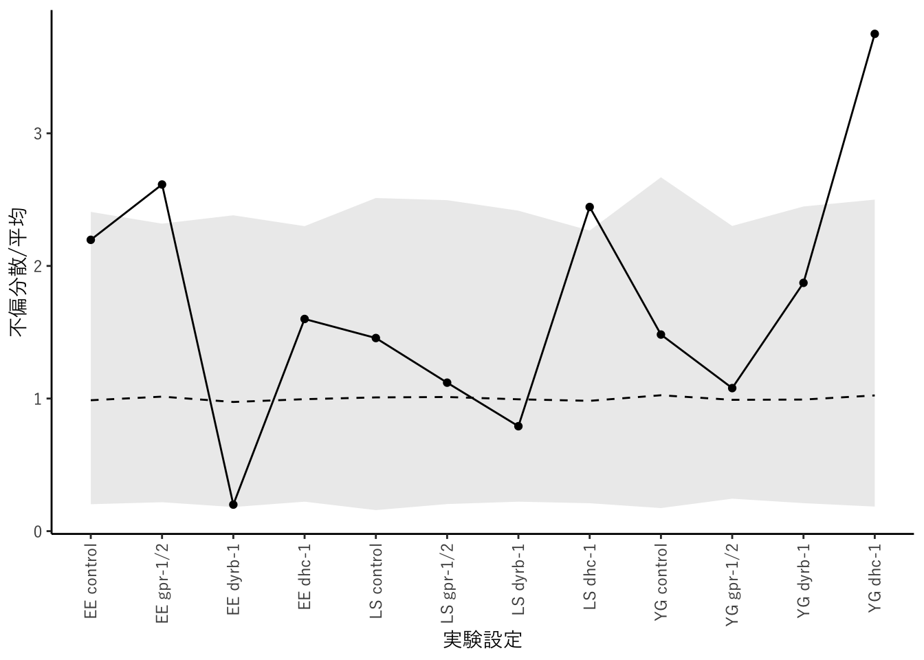
だいたい同じなのですが、95%の領域がいくぶん下にずれているようです。どこか見落としていることがあるかもしれません。
花の数のデータ
スズランの葉の長さと果実の数のデータですが、全部のデータは不明ですので、だいたいおなじようなデータを乱数を使って生成しました。あとで過分散があることがわかりますので、負の二項分布にしたがう乱数を使用しました。
alpha <- -0.798
beta <- 0.101

n <- 60

x <- runif(n, 8, 23)
y <- rnbinom(n, mu = exp(alpha + beta * x), size = 7.5)

df <- data.frame(x = x, y = y)

p1 <- ggplot(df, aes(x = x, y = y)) +
  geom_point(size = 2) +
  scale_x_continuous(name = "葉の長さ (cm)",
                     limits = c(5, 25),
                     breaks = seq(5, 25, 5)) +
  scale_y_continuous(name = "果実数",
                     limits = c(-1, 12),
                     breaks = seq(0, 12, 2)) +
  theme_bw(base_family = jp_font)
plot(p1)
回帰
そのまま線形回帰を適用した場合です。
fit_lm <- lm(y ~ x, data = df)
summary(fit_lm)
##
## Call:
## lm(formula = y ~ x, data = df)
##
## Residuals:
##     Min      1Q  Median      3Q     Max
## -2.5691 -1.0033 -0.3791  0.5319  6.5733
##
## Coefficients:
##             Estimate Std. Error t value Pr(>|t|)
## (Intercept) -0.63961    0.75285  -0.850 0.399051
## x            0.18520    0.04662   3.972 0.000199 ***
## ---
## Signif. codes:  0 '***' 0.001 '**' 0.01 '*' 0.05 '.' 0.1 ' ' 1
##
## Residual standard error: 1.728 on 58 degrees of freedom
## Multiple R-squared:  0.2139, Adjusted R-squared:  0.2003
## F-statistic: 15.78 on 1 and 58 DF,  p-value: 0.0001992
グラフにします(図3.2)。
alpha_hat <- coef(fit_lm)["(Intercept)"]
beta_hat <- coef(fit_lm)["x"]
x_seg <- c(5, min(df$x), max(df$x), 25)
y_seg <- alpha_hat + beta_hat * x_seg

p1 +
  annotate("segment", x = x_seg[1], y = y_seg[1],
           xend = x_seg[2], yend = y_seg[2], linetype = 2) +
  annotate("segment", x = x_seg[2], y = y_seg[2],
           xend = x_seg[3], yend = y_seg[3], linetype = 1) +
  annotate("segment", x = x_seg[3], y = y_seg[3],
           xend = x_seg[4], yend = y_seg[4], linetype = 2)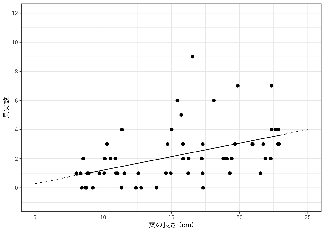
ポアソン回帰です。
fit_glm <- glm(y ~ x, family = poisson(link = log), data = df)
summary(fit_glm)
##
## Call:
## glm(formula = y ~ x, family = poisson(link = log), data = df)
##
## Coefficients:
##             Estimate Std. Error z value Pr(>|z|)
## (Intercept) -0.62017    0.34204  -1.813   0.0698 .
## x            0.08638    0.01909   4.525 6.03e-06 ***
## ---
## Signif. codes:  0 '***' 0.001 '**' 0.01 '*' 0.05 '.' 0.1 ' ' 1
##
## (Dispersion parameter for poisson family taken to be 1)
##
##     Null deviance: 98.807  on 59  degrees of freedom
## Residual deviance: 77.222  on 58  degrees of freedom
## AIC: 217.91
##
## Number of Fisher Scoring iterations: 5
切片だけのモデルです。
fit_glm0 <- glm(y ~ 1, family = poisson(link = log), data = df)
summary(fit_glm0)
##
## Call:
## glm(formula = y ~ 1, family = poisson(link = log), data = df)
##
## Coefficients:
##             Estimate Std. Error z value Pr(>|z|)
## (Intercept)  0.79600    0.08671    9.18   <2e-16 ***
## ---
## Signif. codes:  0 '***' 0.001 '**' 0.01 '*' 0.05 '.' 0.1 ' ' 1
##
## (Dispersion parameter for poisson family taken to be 1)
##
##     Null deviance: 98.807  on 59  degrees of freedom
## Residual deviance: 98.807  on 59  degrees of freedom
## AIC: 237.5
##
## Number of Fisher Scoring iterations: 5
図示します(図3.3)。
alpha_hat <- coef(fit_glm)["(Intercept)"]
beta_hat <- coef(fit_glm)["x"]
alpha0_hat <- coef(fit_glm0)["(Intercept)"]
x_new <- seq(min(df$x), max(df$x), length = 101)
y_new <- exp(alpha_hat + beta_hat * x_new)
y0_new <- exp(alpha0_hat + 0 * x_new)
df_new <- data.frame(x = x_new, y = y_new, y0 = y0_new)

p2 <- p1 +
  geom_line(data = df_new,
            mapping = aes(x = x, y = y)) +
  geom_line(data = df_new,
            mapping = aes(x = x, y = y0), linetype = 2)
plot(p2)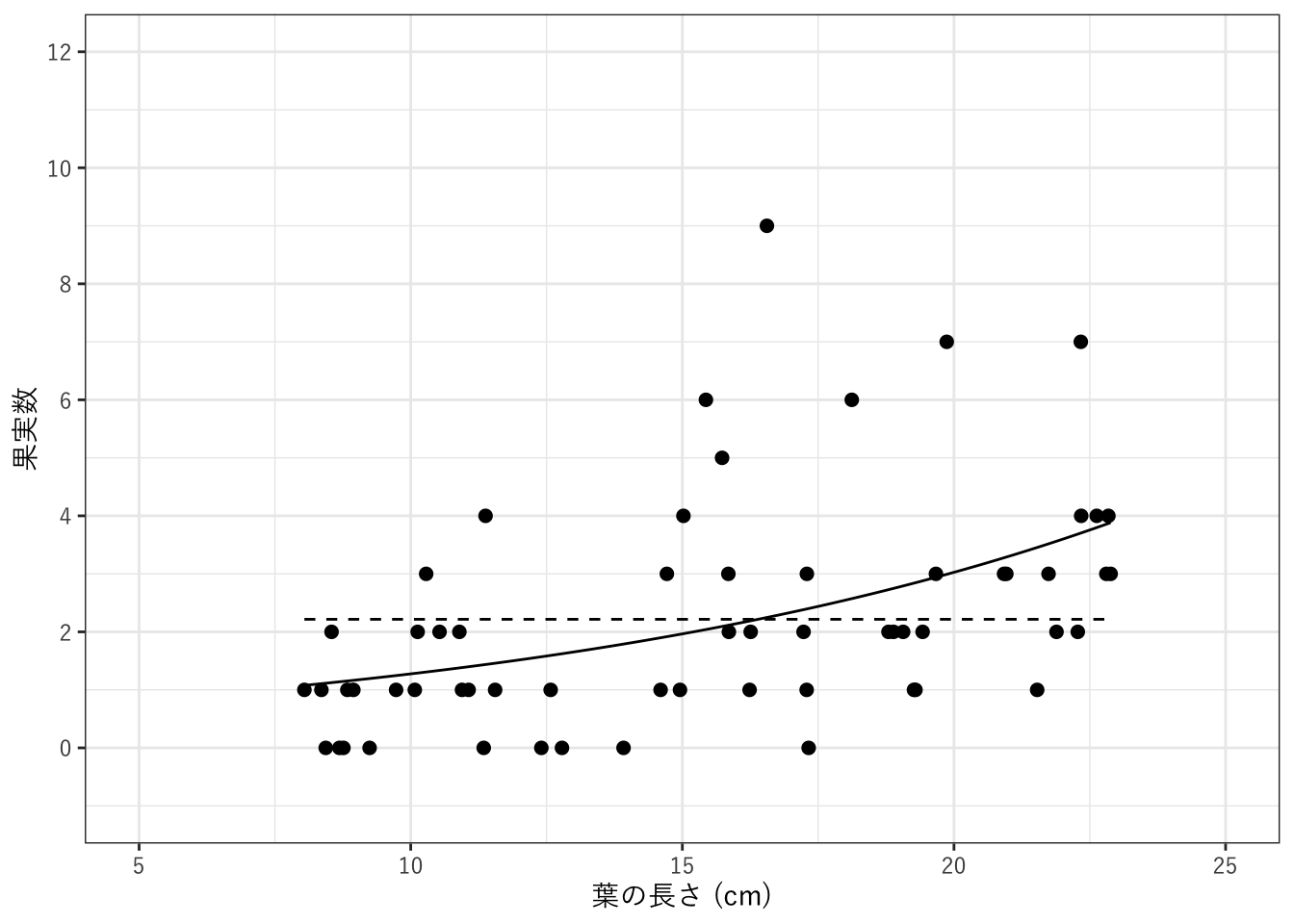
シミュレーションによる検証
ポアソン回帰で推定されたパラメータを用いて、データを再現できるか検証します。図3.5に相当する図を作図します。曲線が回帰曲線、横線が各データ点に対する上下95%の値、点が元データの値です。
sim_fun <- function(x, alpha, beta) {
  rpois(length(x), exp(alpha + beta * x))
}

R <- 1000
sim_result <- replicate(R, sim_fun(x, alpha_hat, beta_hat)) |>
  apply(1, quantile, probs = c(0.025, 0.975))
sim_df <- data.frame(x = x,
                     lower = sim_result["2.5%", ],
                     upper = sim_result["97.5%", ])
p2 +
  geom_segment(data = sim_df,
               mapping = aes(x = x - 0.25, xend = x + 0.25,
                             y = lower),
               colour = "black", alpha = 0.5) +
  geom_segment(data = sim_df,
               mapping = aes(x = x - 0.25, xend = x + 0.25,
                             y = upper),
               colour = "black", alpha = 0.5)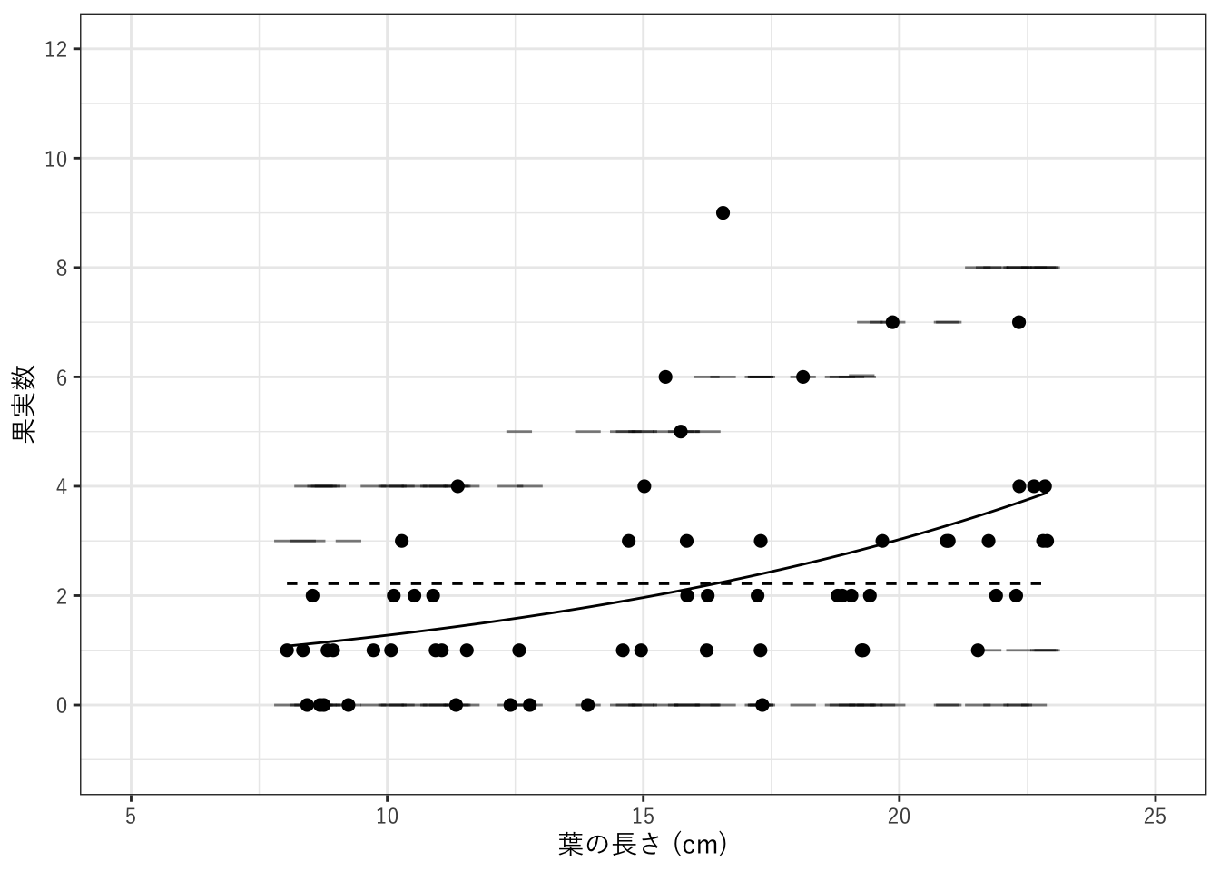
設定どおり、いくつかの点が95%区間からはずれます。
おわりに
ポアソン分布でデータを説明できないところがありましたが、このあてはまっていないところに適切な解釈を与えるような新しいモデルを考案し、さらに検証すべし、というのが著者のメッセージになっています。