library(gamlss)
## Loading required package: splines
## Loading required package: gamlss.data
##
## Attaching package: 'gamlss.data'
## The following object is masked from 'package:datasets':
##
##     sleep
## Loading required package: gamlss.dist
## Loading required package: nlme
## Loading required package: parallel
##  **********   GAMLSS Version 5.5-0  **********
## For more on GAMLSS look at https://www.gamlss.com/
## Type gamlssNews() to see new features/changes/bug fixes.
library(ggplot2)R研究集会2025での安川武彦さんの発表「Rでできる分布回帰のいろいろ」で、GAMLSS (Generalized Additive Models for Location Scale and Shape)とRの[gamlss[(https://cran.r-project.org/package=gamlss)パッケージのことを知りました。期待値だけではなく、分散や歪度、尖度などもモデル化して、あてはめるというものです。さっそく試してみました。
準備
gamlssパッケージと、グラフ作成のためにggplot2パッケージを読み込みます。
データ
gamlssパッケージに含まれるabdomデータを使います。妊娠週数(x)と胎児の腹囲(y, mm)のデータです。
data(abdom)
head(abdom)
##    y     x
## 1 59 12.29
## 2 64 12.29
## 3 56 12.29
## 4 61 12.43
## 5 74 12.71
## 6 60 12.71
まずはデータをプロットしてみます。
ggplot(abdom, aes(x = x, y = y)) +
  geom_point() +
  labs(x = "Gestational age (weeks)",
       y = "Abdominal circumference (mm)")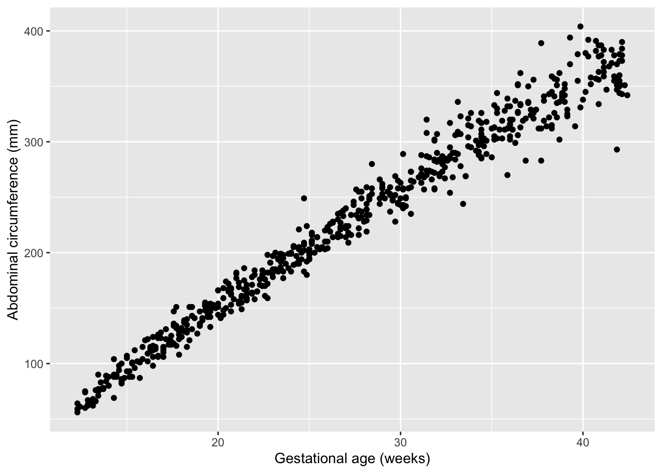
xがおおきくなるにつれて、yのばらつきもおおきくなっているようです。
モデルあてはめ
線形モデル
まずは通常の線形モデルをあてはめてみます。
fit_lm <- lm(y ~ x, data = abdom)
summary(fit_lm)
##
## Call:
## lm(formula = y ~ x, data = abdom)
##
## Residuals:
##     Min      1Q  Median      3Q     Max
## -84.579  -8.105  -0.185   8.064  54.325
##
## Coefficients:
##             Estimate Std. Error t value Pr(>|t|)
## (Intercept) -55.1795     2.0010  -27.58   <2e-16 ***
## x            10.3382     0.0701  147.49   <2e-16 ***
## ---
## Signif. codes:  0 '***' 0.001 '**' 0.01 '*' 0.05 '.' 0.1 ' ' 1
##
## Residual standard error: 14.63 on 608 degrees of freedom
## Multiple R-squared:  0.9728, Adjusted R-squared:  0.9728
## F-statistic: 2.175e+04 on 1 and 608 DF,  p-value: < 2.2e-16
AICの値も見てみます。
AIC(fit_lm)
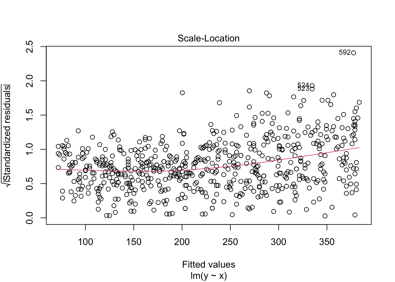
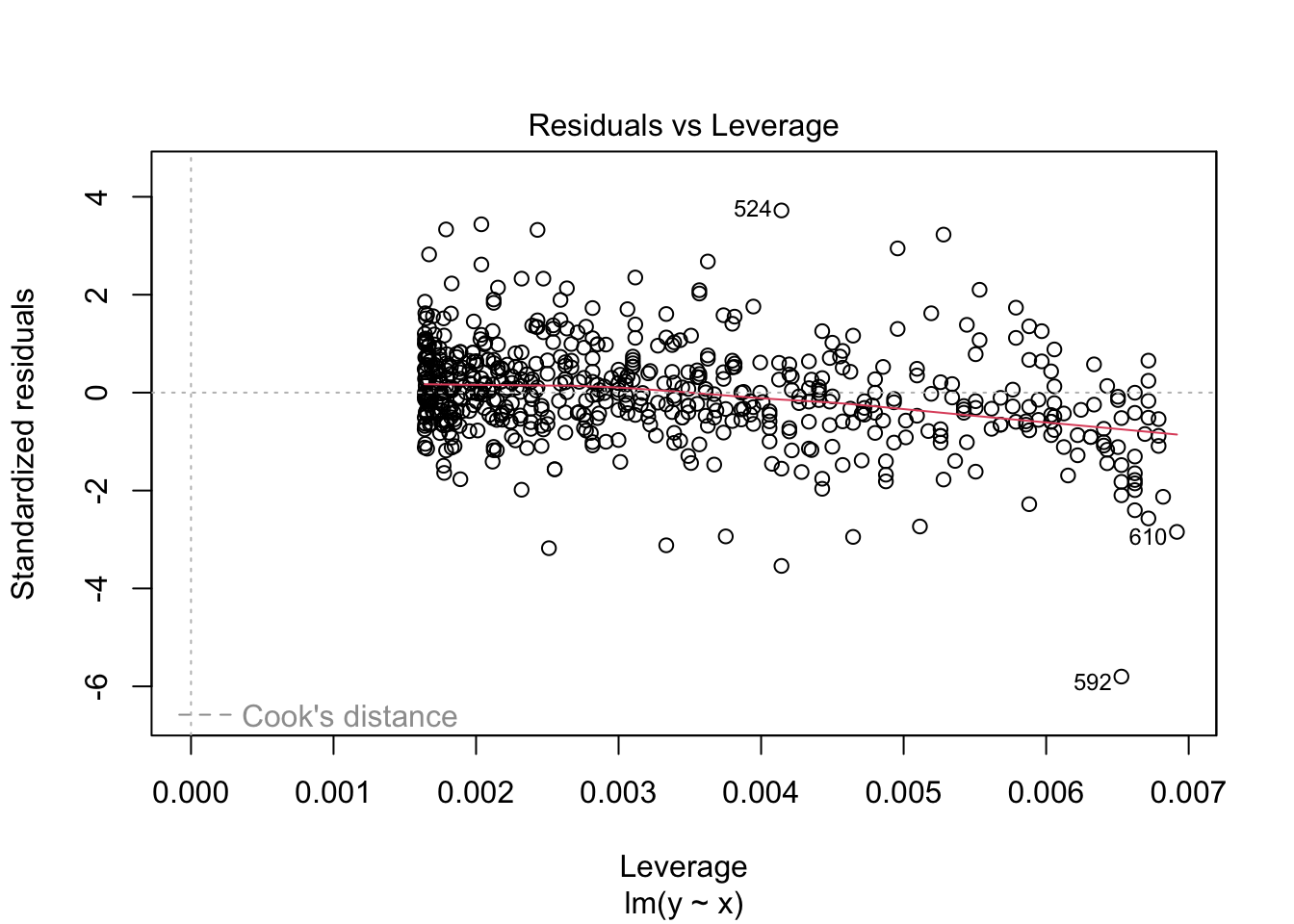
## [1] 5008.453診断プロットを作成します。これは線形回帰モデルの診断でも紹介したものです。上から、残差プロット、正規Q-Qプロット、標準化残差の絶対値の平方根プロット、てこ比と標準化残差との関係とCookの距離を示したプロットになります。
plot(fit_lm, ask = FALSE)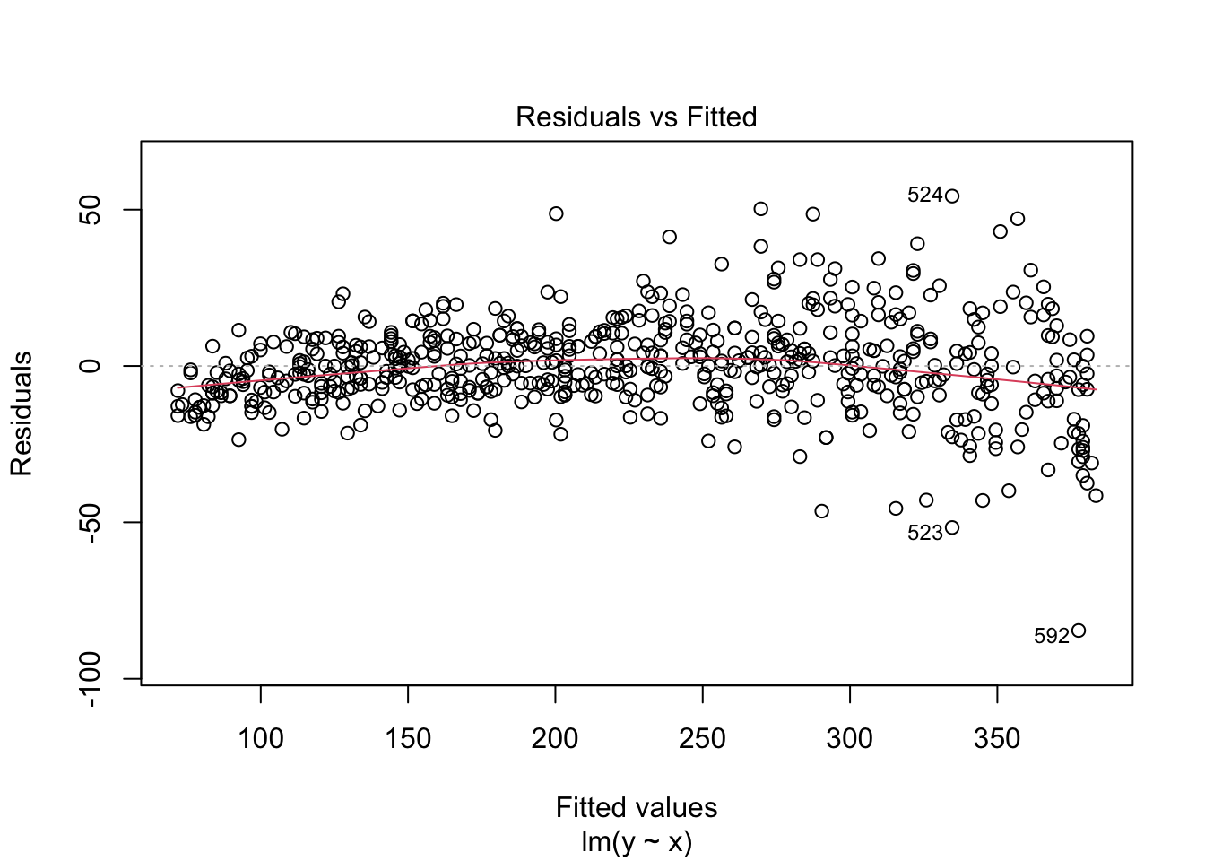
ggplot2でも、残差プロットと正規Q-Qプロットを作成してみます。
ggplot(abdom, aes(x = fitted(fit_lm), y = resid(fit_lm))) +
  geom_point() +
  geom_hline(yintercept = 0, linetype = "dashed") +
  labs(x = "Fitted values",
       y = "Residuals")
値が大きくなるにつれて、残差のばらつきが大きくなっています。
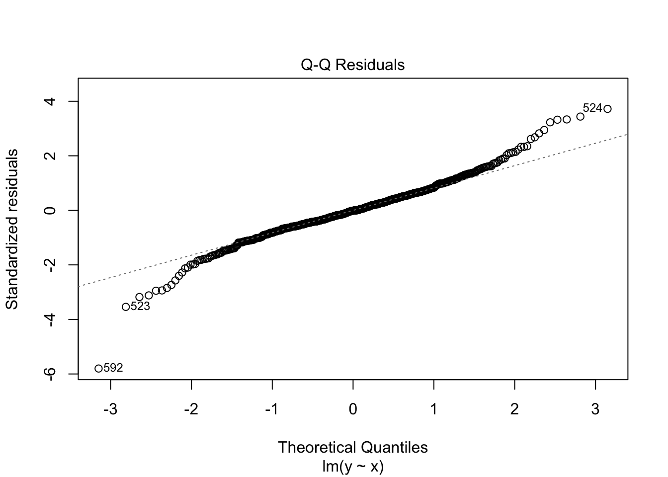
ggplot(abdom, aes(sample = scale(resid(fit_lm)))) +
  stat_qq() +
  stat_qq_line() +
  labs(x = "Theoretical Quantiles",
       y = "Standardized Residuals")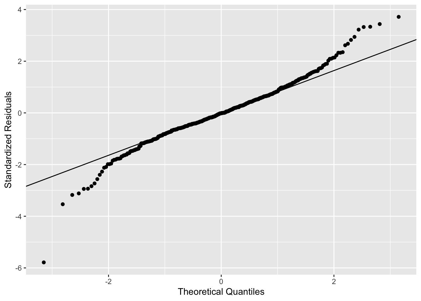
Q-Qプロットを見ると、両端で外れ具合が大きくなっているのがわかります。
GAMLSS
つづいて、GAMLSSであてはめをおこないます。期待値はxのスプライン関数(pb)、分散もxのスプライン関数(pb)でモデル化します。分布はBox-Cox t分布(BCT)を使います。method引数はアルゴリズムの指定で、ここではRigby and StasinopoulosとCole and Greenを組み合わせるようにしています。このあたりは、オンラインマニュアルの例題そのままです。
fit_gamlss <- gamlss(y ~ pb(x), sigma.formula = ~pb(x),
              family = BCT, data = abdom,
              method = mixed(1, 20))
## GAMLSS-RS iteration 1: Global Deviance = 4771.925
## GAMLSS-CG iteration 1: Global Deviance = 4771.013
## GAMLSS-CG iteration 2: Global Deviance = 4770.994
## GAMLSS-CG iteration 3: Global Deviance = 4770.994
summary(fit_gamlss)
## ******************************************************************
## Family:  c("BCT", "Box-Cox t")
##
## Call:  gamlss(formula = y ~ pb(x), sigma.formula = ~pb(x),
##     family = BCT, data = abdom, method = mixed(1, 20))
##
## Fitting method: mixed(1, 20)
##
## ------------------------------------------------------------------
## Mu link function:  identity
## Mu Coefficients:
##              Estimate Std. Error t value Pr(>|t|)
## (Intercept) -64.44299    1.33397  -48.31   <2e-16 ***
## pb(x)        10.69464    0.05787  184.80   <2e-16 ***
## ---
## Signif. codes:  0 '***' 0.001 '**' 0.01 '*' 0.05 '.' 0.1 ' ' 1
##
## ------------------------------------------------------------------
## Sigma link function:  log
## Sigma Coefficients:
##             Estimate Std. Error t value Pr(>|t|)
## (Intercept) -2.65041    0.10859 -24.407  < 2e-16 ***
## pb(x)       -0.01002    0.00380  -2.638  0.00855 **
## ---
## Signif. codes:  0 '***' 0.001 '**' 0.01 '*' 0.05 '.' 0.1 ' ' 1
##
## ------------------------------------------------------------------
## Nu link function:  identity
## Nu Coefficients:
##             Estimate Std. Error t value Pr(>|t|)
## (Intercept)  -0.1072     0.6296   -0.17    0.865
##
## ------------------------------------------------------------------
## Tau link function:  log
## Tau Coefficients:
##             Estimate Std. Error t value Pr(>|t|)
## (Intercept)   2.4948     0.4261   5.855 7.86e-09 ***
## ---
## Signif. codes:  0 '***' 0.001 '**' 0.01 '*' 0.05 '.' 0.1 ' ' 1
##
## ------------------------------------------------------------------
## NOTE: Additive smoothing terms exist in the formulas:
##  i) Std. Error for smoothers are for the linear effect only.
## ii) Std. Error for the linear terms maybe are not accurate.
## ------------------------------------------------------------------
## No. of observations in the fit:  610
## Degrees of Freedom for the fit:  11.7603
##       Residual Deg. of Freedom:  598.2397
##                       at cycle:  3
##
## Global Deviance:     4770.994
##             AIC:     4794.515
##             SBC:     4846.419
## ******************************************************************
AICの値は線形モデルよりも小さくなっていました。
診断プロットです。
plot(fit_gamlss)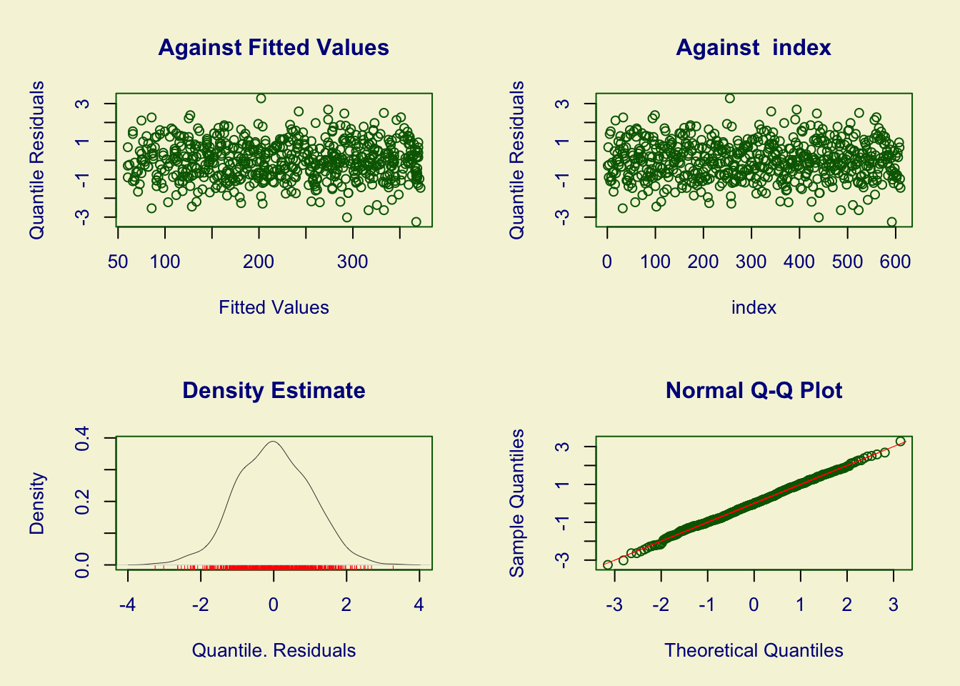
## ******************************************************************
##        Summary of the Quantile Residuals
##                            mean   =  0.001237747
##                        variance   =  1.001867
##                coef. of skewness  =  -0.004513695
##                coef. of kurtosis  =  2.994576
## Filliben correlation coefficient  =  0.999324
## ******************************************************************
ggplot2でも、Q-Qプロットを作成してみます。
ggplot(abdom, aes(sample = scale(resid(fit_gamlss)))) +
  stat_qq() +
  stat_qq_line() +
  labs(x = "Theoretical Quantiles",
       y = "Sample Quantiles")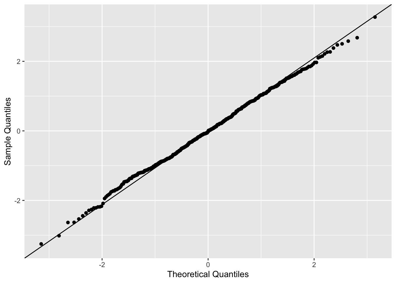
おわりに
GAMLSSについての日本語での解説としては、「GAMLSSとBAMLSSで分布をデータにフィット - 草薙の研究ログ」がありました。こちらでは、単変量の母数の推定と、回帰モデルのあてはめについて解説されています。