install.packages("jmastats")2月28日に開催されたSappoRo.R #13での@tak060237さんの発表「北海道フェノロジー」で紹介されていたjmastatsパッケージを使ってみます。このパッケージは、気象庁が公開している気象観測データをRから取得するというもので、作者は瓜生さんです。瓜生さんによる解説記事(jmastatsパッケージによる気象庁の気象データの取得〜過去100年間の気温のヒートマップを作成するまで〜)もあります。
今回は、札幌・熊谷・金沢・高知の4地点で、2025年の月平均気温と降水量を図示してみました。
インストールと準備
jmastasパッケージはCRANに登録されているので、普通にinstall.packages関数でインストールできます。
インストール後はlibrary関数で読込めます。
また、tidyverseパッケージとunitsパッケージも読込み、対象とする地点も設定しておきます。
library(jmastats)
library(tidyverse)
## ── Attaching core tidyverse packages ──────────────────────── tidyverse 2.0.0 ──
## ✔ dplyr     1.1.4     ✔ readr     2.1.5
## ✔ forcats   1.0.0     ✔ stringr   1.5.2
## ✔ ggplot2   4.0.0     ✔ tibble    3.3.0
## ✔ lubridate 1.9.4     ✔ tidyr     1.3.1
## ✔ purrr     1.1.0
## ── Conflicts ────────────────────────────────────────── tidyverse_conflicts() ──
## ✖ dplyr::filter() masks stats::filter()
## ✖ dplyr::lag()    masks stats::lag()
## ℹ Use the conflicted package (<http://conflicted.r-lib.org/>) to force all conflicts to become errors
library(units)
## udunits database from /Library/Frameworks/R.framework/Versions/4.5-arm64/Resources/library/units/share/udunits/udunits2.xml

locs <- c("札幌", "熊谷", "金沢", "高知")
year <- 2025パッケージに含まれるデータstationsにはアメダス観測点の情報が収録されています。
head(stations, 10)
## Simple feature collection with 10 features and 13 fields
## Geometry type: POINT
## Dimension:     XY
## Bounding box:  xmin: 141.045 ymin: 45.10167 xmax: 142.35 ymax: 45.52
## Geodetic CRS:  WGS 84
## # A tibble: 10 × 14
##    area  station_no station_type station_name address                  elevation
##    <chr>      <int> <chr>        <chr>        <chr>                        <int>
##  1 宗谷       11001 四           宗谷岬       稚内市宗谷岬                    26
##  2 宗谷       11016 官           稚内         稚内市開運 稚内地方気象台……         3
##  3 宗谷       11046 四           礼文         礼文郡礼文町大字香深村トンナイ……        65
##  4 宗谷       11061 官           声問         稚内市大字声問村字声問 稚内航空気象観測所……         8
##  5 宗谷       11076 四           浜鬼志別     宗谷郡猿払村浜鬼志別            13
##  6 宗谷       11091 官           本泊         利尻郡利尻富士町鴛泊字本泊 利尻航空気象観測所…        30
##  7 宗谷       11121 四           沼川         稚内市声問村沼川                23
##  8 宗谷       11151 四           沓形         利尻郡利尻町沓形泉町            14
##  9 宗谷       11176 四           豊富         天塩郡豊富町豊富東2条           14
## 10 宗谷       11206 四           浜頓別       枝幸郡浜頓別町クッチャロ湖畔……        18
## # ℹ 8 more variables: observation_begin <chr>, note1 <chr>, note2 <chr>,
## #   katakana <chr>, prec_no <chr>, block_no <chr>, pref_code <chr>,
## #   geometry <POINT [°]>
データの取得
観測データの取得に必要な、各対象地点のblock_noを取得します。複数の行になっている観測地点もあるので(札幌とか)unique関数で1つにしておきます。取得したlocs_noは、各block_noを値とする文字列ベクトルになりますので、要素の名前に地点名を与えておきます。
locs_no <- stations |>
  dplyr::filter(station_name %in% locs) |>
  dplyr::pull(block_no) |>
  unique()
names(locs_no) <- locsjma_collect関数で観測データを取得します。月ごとのデータを取得しますので、item引数には"monthly"を指定します。また、purrrパッケージのmap関数をつかって、block_no引数にはlocs_noの各要素を与えるようにしています。
その後、purrrパッケージのlist_rbind関数で、map関数から返されたリストをデータフレームにまとめます。このときnames_to引数に"loc"を指定して、loc列に地点名がはいるようにしています。
なお、手もとの環境では、初回にターミナルからmkdir ~/Library/Caches/jmastatsとして、手動でキャッシュディレクトリを作成しておかないとキャッシュが有効になりませんでした。
df <- purrr::map(
  locs_no,
  \(x)
    jma_collect(item = "monthly",
                block_no = x,
                year = year)) |>
  purrr::list_rbind(names_to = "loc")
解説にあるように、このデータはネストされたデータフレームになっています。
glimpse(df)
## Rows: 48
## Columns: 12
## $ loc              <chr> "札幌", "札幌", "札幌", "札幌", "札幌", "札幌", "札幌", "札幌", "札幌",…
## $ month            <dbl> 1, 2, 3, 4, 5, 6, 7, 8, 9, 10, 11, 12, 1, 2, 3, 4, 5,…
## $ atmosphere       <tibble[,2]> <tbl_df[26 x 2]>
## $ precipitation    <tibble[,4]> <tbl_df[26 x 4]>
## $ temperature      <tibble[,5]> <tbl_df[26 x 5]>
## $ humidity         <tibble[,2]> <tbl_df[26 x 2]>
## $ wind             <tibble[,5]> <tbl_df[26 x 5]>
## $ daylight         <tibble[,1]> <tbl_df[26 x 1]>
## $ snow             <tibble[,3]> <tbl_df[26 x 3]>
## $ solar_irradiance <tibble[,1]> <tbl_df[26 x 1]>
## $ cloud_covering   <tibble[,1]> <tbl_df[26 x 1]>
## $ condition <tibble[,3]> <tbl_df[26 x 3]>降水量(precipiation)と気温(temperature)を抽出して、ネストされたデータを展開します。最後に、parse_unit関数で、列名に含まれる単位を除いて、値をunitsオブジェクトに変換します。
df_pt <- df |>
  dplyr::select(loc, month, precipitation, temperature) |>
  tidyr::unnest(c(precipitation, temperature), names_sep = "_") |>
  parse_unit()
このようになります。
glimpse(df_pt)
## Rows: 48
## Columns: 11
## $ loc                         <chr> "札幌", "札幌", "札幌", "札幌", "札幌", "札幌", "札幌", …
## $ month                       <dbl> 1, 2, 3, 4, 5, 6, 7, 8, 9, 10, 11, 12, 1, …
## $ precipitation_sum           [mm] 68.5 [mm], 118.0 [mm], 94.5 [mm], 110.0 [mm…
## $ precipitation_max_per_day   [mm] 18.5 [mm], 17.0 [mm], 16.5 [mm], 30.0 [mm],…
## $ precipitation_max_1hour     [mm] 3.0 [mm], 6.0 [mm], 4.0 [mm], 7.0 [mm], 4.5…
## $ precipitation_max_10minutes [mm] 1.0 [mm], 1.5 [mm], 1.5 [mm], 1.5 [mm], 1.0…
## $ temperature_average         [°C] -1.2 [°C], -0.9 [°C], 2.0 [°C], 8.5 [°C], 1…
## $ temperature_average_max     [°C] 1.5 [°C], 2.4 [°C], 5.3 [°C], 13.0 [°C], 20…
## $ temperature_average_min     [°C] -3.8 [°C], -4.4 [°C], -1.3 [°C], 5.2 [°C], …
## $ temperature_max             [°C] 5.4 [°C], 10.9 [°C], 11.6 [°C], 21.1 [°C], …
## $ temperature_min             [°C] -8.5 [°C], -8.2 [°C], -6.4 [°C], -0.6 [°C],…
可視化
4地点の2025年の月平均気温と最高気温・最低気温の平均、それから月降水量をグラフにします。月平均気温を赤の折れ線で、最高・最低気温の平均を縦線で描画しています。また、降水量を水色の棒グラフにしています。
aes関数のy, ymin, ymax引数に与える値は、units型のままだと異なる単位を混ぜて使えないので、as.numeric関数で数値型にしています。
左のY軸を降水量に、右のY軸を気温としました。降水量600mmと気温30℃とで縦軸の値をあわせるようにしています。
ggplot(df_pt) +
  geom_col(aes(x = month,
               y = as.numeric(precipitation_sum)),
           fill = "lightblue") +
  geom_line(aes(x = month,
                y = as.numeric(temperature_average) / 30 * 600),
            colour = "red") +
  geom_linerange(aes(x = month,
                     ymin = as.numeric(temperature_average_min) / 30 * 600,
                     ymax = as.numeric(temperature_average_max) / 30 * 600),
            colour = "red") +
  scale_x_continuous(name = "月",
                     breaks = 1:12, minor_breaks = NULL) +
  scale_y_continuous(name = "降水量 (mm)",
                     sec.axis = sec_axis(
                       ~ . / 600 * 30,
                       name = "気温(℃)")) +
  facet_wrap(~ loc, ncol = 2) +
  theme_bw(base_family = "Noto Sans JP")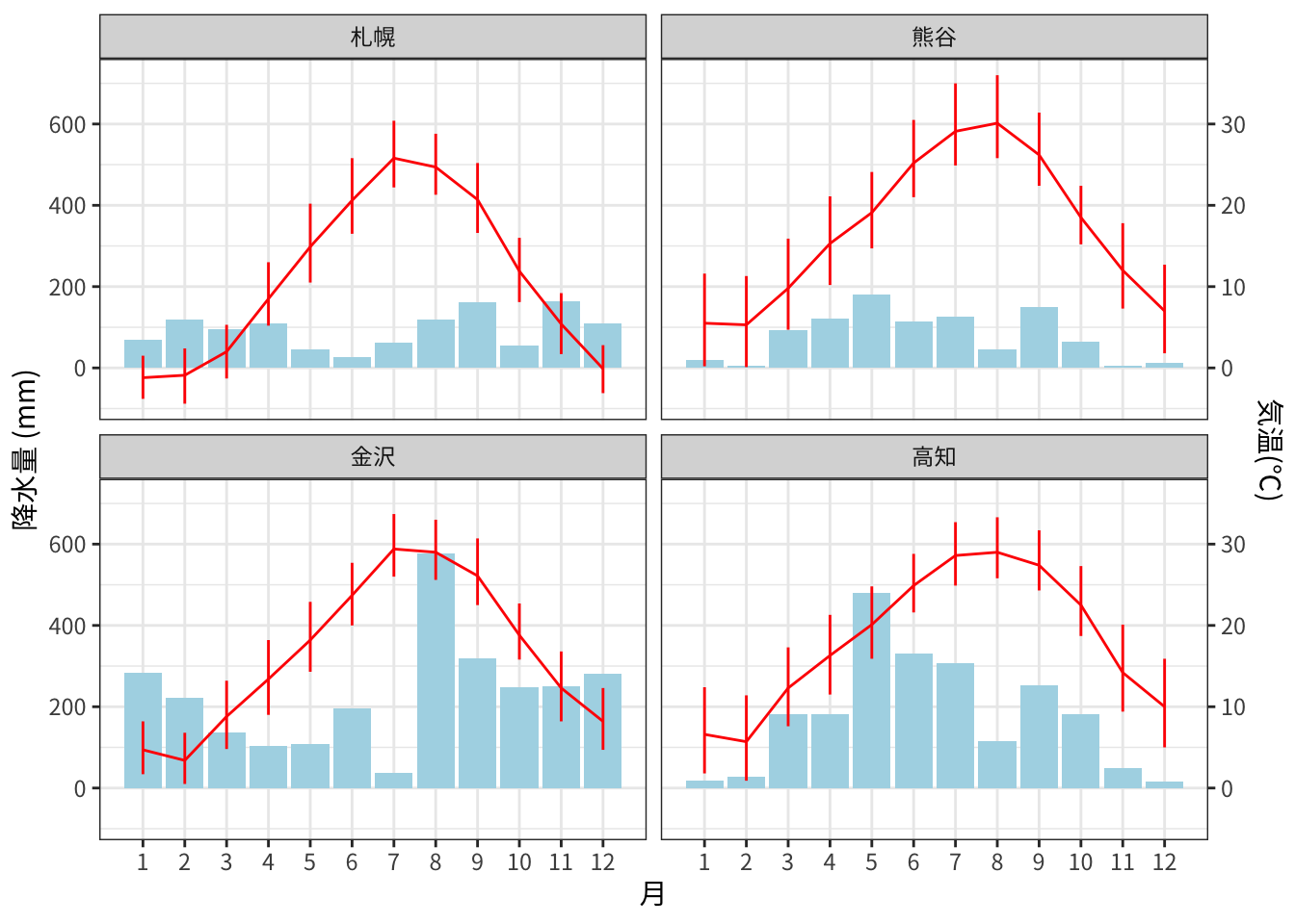
金沢の8月の降水量が多いのは、2025年8月7日の集中豪雨のためです。